snacks.nvim/tests/image/big.md

• chapters 3 to 8 from the book measure theory, by Sheldon Axler. LICENSE

Chapter 3

Integration

To remedy deficiencies of Riemann integration that were discussed in Section 1B, in the last chapter we developed measure theory as an extension of the notion of the length of an interval. Having proved the fundamental results about measures, we are now ready to use measures to develop integration with respect to a measure.

As we will see, this new method of integration fixes many of the problems with Riemann integration. In particular, we will develop good theorems for interchanging limits and integrals.

Statue in Milan of Maria Gaetana Agnesi, who in 1748 published one of the first calculus textbooks. A translation of her book into English was published in 1801. In this chapter, we develop a method of integration more powerful than methods contemplated by the pioneers of calculus.

@Giovanni Dall'Orto

3A Integration with Respect to a Measure

Integration of Nonnegative Functions

We will first define the integral of a nonnegative function with respect to a measure. Then by writing a real-valued function as the difference of two nonnegative functions, we will define the integral of a real-valued function with respect to a measure. We begin this process with the following definition.

3.1 Definition $\mathcal{S}$-partition

Suppose \mathcal{S} is a $\sigma$-algebra on a set X. An $\mathcal{S}$-partition of X is a finite collection A_{1}, \ldots, A_{m} of disjoint sets in \mathcal{S} such that A_{1} \cup \cdots \cup A_{m}=X.

The next definition should remind you of the definition of the lower Riemann sum (see 1.3). However, now we are working with an arbitrary measure and

We adopt the convention that 0 \cdot \infty and \infty \cdot 0 should both be interpreted to be 0 . thus X need not be a subset of \mathbf{R}. More importantly, even in the case when X is a closed interval [a, b] in \mathbf{R} and \mu is Lebesgue measure on the Borel subsets of [a, b], the sets A_{1}, \ldots, A_{m} in the definition below do not need to be subintervals of [a, b] as they do for the lower Riemann sum-they need only be Borel sets.

3.2 Definition lower Lebesgue sum

Suppose (X, \mathcal{S}, \mu) is a measure space, f: X \rightarrow[0, \infty] is an $\mathcal{S}$-measurable function, and P is an $\mathcal{S}$-partition A_{1}, \ldots, A_{m} of X. The lower Lebesgue sum \mathcal{L}(f, P) is defined by

\mathcal{L}(f, P)=\sum_{j=1}^{m} \mu\left(A_{j}\right) \inf {A{j}} f

Suppose (X, \mathcal{S}, \mu) is a measure space. We will denote the integral of an \mathcal{S} measurable function f with respect to \mu by \int f d \mu. Our basic requirements for an integral are that we want \int \chi_{E} d \mu to equal \mu(E) for all E \in \mathcal{S}, and we want \int(f+g) d \mu=\int f d \mu+\int g d \mu. As we will see, the following definition satisfies both of those requirements (although this is not obvious). Think about why the following definition is reasonable in terms of the integral equaling the area under the graph of the function (in the special case of Lebesgue measure on an interval of \mathbf{R} ).

3.3 Definition integral of a nonnegative function

Suppose (X, \mathcal{S}, \mu) is a measure space and f: X \rightarrow[0, \infty] is an $\mathcal{S}$-measurable function. The integral of f with respect to \mu, denoted \int f d \mu, is defined by

\int f d \mu=\sup {\mathcal{L}(f, P): P \text { is an } \mathcal{S} \text {-partition of } X}

Suppose (X, \mathcal{S}, \mu) is a measure space and f: X \rightarrow[0, \infty] is an $\mathcal{S}$-measurable function. Each $\mathcal{S}$-partition A_{1}, \ldots, A_{m} of X leads to an approximation of f from below by the $\mathcal{S}$-measurable simple function \sum_{j=1}^{m}\left(\inf _{A_{j}} f\right) \chi_{A_{j}}. This suggests that

\sum_{j=1}^{m} \mu\left(A_{j}\right) \inf {A{j}} f

should be an approximation from below of our intuitive notion of \int f d \mu. Taking the supremum of these approximations leads to our definition of \int f d \mu.

The following result gives our first example of evaluating an integral.

3.4 integral of a characteristic function

Suppose (X, \mathcal{S}, \mu) is a measure space and E \in \mathcal{S}. Then

\int \chi_{E} d \mu=\mu(E) .

Proof If P is the $\mathcal{S}$-partition of X consisting of E and its complement X \backslash E, then clearly \mathcal{L}\left(\chi_{E}, P\right)=\mu(E). Thus \int \chi_{E} d \mu \geq \mu(E).

To prove the inequality in the other direction, suppose P is an $\mathcal{S}$-partition A_{1}, \ldots, A_{m} of X. Then \mu\left(A_{j}\right) \inf _{A_{j}} \chi_{E} equals \mu\left(A_{j}\right) if A_{j} \subset E and equals 0 otherwise. Thus

\begin{aligned} \mathcal{L}\left(\chi_{E}, P\right) & =\sum_{\left{j: A_{j} \subset E\right}} \mu\left(A_{j}\right) \ & =\mu\left(\bigcup_{\left{j: A_{j} \subset E\right}} A_{j}\right) \ & \leq \mu(E) . \end{aligned}

The symbol d in the expression \int f \mathrm{~d} \mu has no independent meaning, but it often usefully separates f from \mu. Because the d in \int f \mathrm{~d} \mu does not represent another object, some mathematicians prefer typesetting an upright \mathrm{d} in this situation, producing \int f \mathrm{~d} \mu. However, the upright \mathrm{d} looks jarring to some readers who are accustomed to italicized symbols. This book takes the compromise position of using slanted d instead of math-mode italicized d in integrals.

Thus \int \chi_{E} d \mu \leq \mu(E), completing the proof.

3.5 Example integrals of \chi_{\mathbf{Q}} and \chi_{[0,1] \backslash \mathbf{Q}}

Suppose \lambda is Lebesgue measure on \mathbf{R}. As a special case of the result above, we have \int \chi_{\mathbf{Q}} d \lambda=0 (because |\mathbf{Q}|=0 ). Recall that \chi_{\mathbf{Q}} is not Riemann integrable on [0,1]. Thus even at this early stage in our development of integration with respect to a measure, we have fixed one of the deficiencies of Riemann integration.

Note also that 3.4 implies that \int \chi_{[0,1] \backslash \mathbf{Q}} d \lambda=1 (because |[0,1] \backslash \mathbf{Q}|=1 ), which is what we want. In contrast, the lower Riemann integral of \chi_{[0,1] \backslash \mathbf{Q}} on [0,1] equals 0 , which is not what we want.

3.6 Example integration with respect to counting measure is summation

Suppose \mu is counting measure on $\mathbf{Z}^{+}$and b_{1}, b_{2}, \ldots is a sequence of nonnegative numbers. Think of b as the function from $\mathbf{Z}^{+}$to [0, \infty) defined by b(k)=b_{k}. Then

\int b d \mu=\sum_{k=1}^{\infty} b_{k}

as you should verify.

Integration with respect to a measure can be called Lebesgue integration. The next result shows that Lebesgue integration behaves as expected on simple functions represented as linear combinations of characteristic functions of disjoint sets.

3.7 integral of a simple function

Suppose (X, \mathcal{S}, \mu) is a measure space, E_{1}, \ldots, E_{n} are disjoint sets in \mathcal{S}, and c_{1}, \ldots, c_{n} \in[0, \infty]. Then

\int\left(\sum_{k=1}^{n} c_{k} \chi_{E_{k}}\right) d \mu=\sum_{k=1}^{n} c_{k} \mu\left(E_{k}\right)

Proof Without loss of generality, we can assume that E_{1}, \ldots, E_{n} is an $\mathcal{S}$-partition of X [by replacing n by n+1 and setting E_{n+1}=X \backslash\left(E_{1} \cup \ldots \cup E_{n}\right) and c_{n+1}=0 ].

If P is the $\mathcal{S}$-partition E_{1}, \ldots, E_{n} of X, then \mathcal{L}\left(\sum_{k=1}^{n} c_{k} \chi_{E_{k}}{ }^{\prime} P\right)=\sum_{k=1}^{n} c_{k} \mu\left(E_{k}\right). Thus

\int\left(\sum_{k=1}^{n} c_{k} \chi_{E_{k}}\right) d \mu \geq \sum_{k=1}^{n} c_{k} \mu\left(E_{k}\right)

To prove the inequality in the other direction, suppose that P is an $\mathcal{S}$-partition A_{1}, \ldots, A_{m} of X. Then

\begin{aligned} \mathcal{L}\left(\sum_{k=1}^{n} c_{k} \chi_{E_{k}}, P\right) & =\sum_{j=1}^{m} \mu\left(A_{j}\right) \min {\left{i: A{j} \cap E_{i} \neq \varnothing\right}} c_{i} \ & =\sum_{j=1}^{m} \sum_{k=1}^{n} \mu\left(A_{j} \cap E_{k}\right){\left{i: A{j} \cap E_{i} \neq \varnothing\right}} c_{i} \ & \leq \sum_{j=1}^{m} \sum_{k=1}^{n} \mu\left(A_{j} \cap E_{k}\right) c_{k} \ & =\sum_{k=1}^{n} c_{k} \sum_{j=1}^{m} \mu\left(A_{j} \cap E_{k}\right) \ & =\sum_{k=1}^{n} c_{k} \mu\left(E_{k}\right) . \end{aligned}

The inequality above implies that \int\left(\sum_{k=1}^{n} c_{k} \chi_{E_{k}}\right) d \mu \leq \sum_{k=1}^{n} c_{k} \mu\left(E_{k}\right), completing the proof.

The next easy result gives an unsurprising property of integrals.

3.8 integration is order preserving

Suppose (X, \mathcal{S}, \mu) is a measure space and f, g: X \rightarrow[0, \infty] are $\mathcal{S}$-measurable functions such that f(x) \leq g(x) for all x \in X. Then \int f \mathrm{~d} \mu \leq \int g d \mu.

Proof Suppose P is an $\mathcal{S}$-partition A_{1}, \ldots, A_{m} of X. Then

\inf {A{j}} f \leq \inf {A{j}} g

for each j=1, \ldots, m. Thus \mathcal{L}(f, P) \leq \mathcal{L}(g, P). Hence \int f d \mu \leq \int g d \mu.

Monotone Convergence Theorem

For the proof of the Monotone Convergence Theorem (and several other results), we will need to use the following mild restatement of the definition of the integral of a nonnegative function.

3.9 integrals via simple functions

Suppose (X, \mathcal{S}, \mu) is a measure space and f: X \rightarrow[0, \infty] is $\mathcal{S}$-measurable. Then

3.10 \int f d \mu=\sup \left\{\sum_{j=1}^{m} c_{j} \mu\left(A_{j}\right): A_{1}, \ldots, A_{m}\right. are disjoint sets in \mathcal{S},

\begin{aligned} & c_{1}, \ldots, c_{m} \in[0, \infty), \text { and } \ & \left.f(x) \geq \sum_{j=1}^{m} c_{j} \chi_{A_{j}}(x) \text { for every } x \in X\right} \end{aligned}

Proof First note that the left side of 3.10 is bigger than or equal to the right side by 3.7 and 3.8 .

To prove that the right side of 3.10 is bigger than or equal to the left side, first assume that \inf _{A} f<\infty for every A \in \mathcal{S} with \mu(A)>0. Then for P an $\mathcal{S}$-partition A_{1}, \ldots, A_{m} of nonempty subsets of X, take c_{j}=\inf _{A_{j}} f, which shows that \mathcal{L}(f, P) is in the set on the right side of 3.10. Thus the definition of \int f d \mu shows that the right side of 3.10 is bigger than or equal to the left side.

The only remaining case to consider is when there exists a set A \in \mathcal{S} such that \mu(A)>0 and \inf _{A} f=\infty [which implies that f(x)=\infty for all x \in A ]. In this case, for arbitrary t \in(0, \infty) we can take m=1, A_{1}=A, and c_{1}=t. These choices show that the right side of 3.10 is at least t \mu(A). Because t is an arbitrary positive number, this shows that the right side of 3.10 equals \infty, which of course is greater than or equal to the left side, completing the proof.

The next result allows us to interchange limits and integrals in certain circumstances. We will see more theorems of this nature in the next section.

3.11 Monotone Convergence Theorem

Suppose (X, \mathcal{S}, \mu) is a measure space and 0 \leq f_{1} \leq f_{2} \leq \cdots is an increasing sequence of $\mathcal{S}$-measurable functions. Define f: X \rightarrow[0, \infty] by

f(x)=\lim {k \rightarrow \infty} f{k}(x)

Then

\lim {k \rightarrow \infty} \int f{k} d \mu=\int f d \mu

Proof The function f is $\mathcal{S}$-measurable by 2.53 .

Because f_{k}(x) \leq f(x) for every x \in X, we have \int f_{k} d \mu \leq \int f d \mu for each $k \in \mathbf{Z}^{+}$(by 3.8). Thus \lim _{k \rightarrow \infty} \int f_{k} d \mu \leq \int f d \mu.

To prove the inequality in the other direction, suppose A_{1}, \ldots, A_{m} are disjoint sets in \mathcal{S} and c_{1}, \ldots, c_{m} \in[0, \infty) are such that

f(x) \geq \sum_{j=1}^{m} c_{j} \chi_{A_{j}}(x) \quad \text { for every } x \in X

Let t \in(0,1). For k \in \mathbf{Z}^{+}, let

E_{k}=\left{x \in X: f_{k}(x) \geq t \sum_{j=1}^{m} c_{j} \chi_{A_{j}}(x)\right}

Then E_{1} \subset E_{2} \subset \cdots is an increasing sequence of sets in \mathcal{S} whose union equals X. Thus \lim _{k \rightarrow \infty} \mu\left(A_{j} \cap E_{k}\right)=\mu\left(A_{j}\right) for each j \in\{1, \ldots, m\} (by 2.59).

If k \in \mathbf{Z}^{+}, then

f_{k}(x) \geq \sum_{j=1}^{m} t c_{j} \chi_{A_{j} \cap E_{k}}(x)

for every x \in X. Thus (by 3.9)

\int f_{k} d \mu \geq t \sum_{j=1}^{m} c_{j} \mu\left(A_{j} \cap E_{k}\right)

Taking the limit as k \rightarrow \infty of both sides of the inequality above gives

\lim {k \rightarrow \infty} \int f{k} d \mu \geq t \sum_{j=1}^{m} c_{j} \mu\left(A_{j}\right)

Now taking the limit as t increases to 1 shows that

\lim {k \rightarrow \infty} \int f{k} d \mu \geq \sum_{j=1}^{m} c_{j} \mu\left(A_{j}\right)

Taking the supremum of the inequality above over all $\mathcal{S}$-partitions A_{1}, \ldots, A_{m} of X and all c_{1}, \ldots, c_{m} \in[0, \infty ) satisfying 3.12 shows (using 3.9) that we have \lim _{k \rightarrow \infty} \int f_{k} d \mu \geq \int f d \mu, completing the proof.

The proof that the integral is additive will use the Monotone Convergence Theorem and our next result. The representation of a simple function h: X \rightarrow[0, \infty] in the form \sum_{k=1}^{n} c_{k} \chi_{E_{k}} is not unique. Requiring the numbers c_{1}, \ldots, c_{n} to be distinct and E_{1}, \ldots, E_{n} to be nonempty and disjoint with E_{1} \cup \cdots \cup E_{n}=X produces what is called the standard representation of a simple function [take E_{k}=h^{-1}\left(\left\{c_{k}\right\}\right), where c_{1}, \ldots, c_{n} are the distinct values of \left.h\right]. The following lemma shows that all representations (including representations with sets that are not disjoint) of a simple measurable function give the same sum that we expect from integration.

3.13 integral-type sums for simple functions

Suppose (X, \mathcal{S}, \mu) is a measure space. Suppose a_{1}, \ldots, a_{m}, b_{1}, \ldots, b_{n} \in[0, \infty] and A_{1}, \ldots, A_{m}, B_{1}, \ldots, B_{n} \in \mathcal{S} are such that \sum_{j=1}^{m} a_{j} \chi_{A_{j}}=\sum_{k=1}^{n} b_{k} \chi_{B_{k}}. Then

\sum_{j=1}^{m} a_{j} \mu\left(A_{j}\right)=\sum_{k=1}^{n} b_{k} \mu\left(B_{k}\right)

Proof We assume A_{1} \cup \cdots \cup A_{m}=X (otherwise add the term 0 \chi_{X \backslash\left(A_{1} \cup \cdots \cup A_{m}\right.} ). Suppose A_{1} and A_{2} are not disjoint. Then we can write

3.14

a_{1} \chi_{A_{1}}+a_{2} \chi_{A_{2}}=a_{1} \chi_{A_{1} \backslash A_{2}}+a_{2} \chi_{A_{2} \backslash A_{1}}+\left(a_{1}+a_{2}\right) \chi_{A_{1} \cap A_{2}},

where the three sets appearing on the right side of the equation above are disjoint.

Now A_{1}=\left(A_{1} \backslash A_{2}\right) \cup\left(A_{1} \cap A_{2}\right) and A_{2}=\left(A_{2} \backslash A_{1}\right) \cup\left(A_{1} \cap A_{2}\right); each of these unions is a disjoint union. Thus \mu\left(A_{1}\right)=\mu\left(A_{1} \backslash A_{2}\right)+\mu\left(A_{1} \cap A_{2}\right) and \mu\left(A_{2}\right)=\mu\left(A_{2} \backslash A_{1}\right)+\mu\left(A_{1} \cap A_{2}\right). Hence

a_{1} \mu\left(A_{1}\right)+a_{2} \mu\left(A_{2}\right)=a_{1} \mu\left(A_{1} \backslash A_{2}\right)+a_{2} \mu\left(A_{2} \backslash A_{1}\right)+\left(a_{1}+a_{2}\right) \mu\left(A_{1} \cap A_{2}\right) .

The equation above, in conjunction with 3.14 , shows that if we replace the two sets A_{1}, A_{2} by the three disjoint sets A_{1} \backslash A_{2}, A_{2} \backslash A_{1}, A_{1} \cap A_{2} and make the appropriate adjustments to the coefficients a_{1}, \ldots, a_{m}, then the value of the sum \sum_{j=1}^{m} a_{j} \mu\left(A_{j}\right) is unchanged (although m has increased by 1 ).

Repeating this process with all pairs of subsets among A_{1}, \ldots, A_{m} that are not disjoint after each step, in a finite number of steps we can convert the initial list A_{1}, \ldots, A_{m} into a disjoint list of subsets without changing the value of \sum_{j=1}^{m} a_{j} \mu\left(A_{j}\right).

The next step is to make the numbers a_{1}, \ldots, a_{m} distinct. This is done by replacing the sets corresponding to each a_{j} by the union of those sets, and using finite additivity of the measure \mu to show that the value of the sum \sum_{j=1}^{m} a_{j} \mu\left(A_{j}\right) does not change.

Finally, drop any terms for which A_{j}=\varnothing, getting the standard representation for a simple function. We have now shown that the original value of \sum_{j=1}^{m} a_{j} \mu\left(A_{j}\right) is equal to the value if we use the standard representation of the simple function \sum_{j=1}^{m} a_{j} \chi_{A_{j}}. The same procedure can be used with the representation \sum_{k=1}^{n} b_{k} \chi_{B_{k}} to show that \sum_{k=1}^{n} b_{k} \mu\left(\chi_{B_{k}}\right) equals what we would get with the standard representation. Thus the equality of the functions \sum_{j=1}^{m} a_{j} \chi_{A_{j}} and \sum_{k=1}^{n} b_{k} \chi_{B_{k}} implies the equality \sum_{j=1}^{m} a_{j} \mu\left(A_{j}\right)=\sum_{k=1}^{n} b_{k} \mu\left(B_{k}\right).

Now we can show that our definition of integration does the right thing with simple measurable functions that might not be expressed in the standard representation. The result below differs from 3.7 mainly because the sets E_{1}, \ldots, E_{n} in the result below are not required to be disjoint. Like the previous result, the next result would follow immediately from the linearity of integration if that property had already been proved.

If we had already proved that integration is linear, then we could quickly get the conclusion of the previous result by integrating both sides of the equation \sum_{j=1}^{m} a_{j} \chi_{A_{j}}=\sum_{k=1}^{n} b_{k} \chi_{B_{k}} with respect to \mu. However, we need the previous result to prove the next result, which is used in our proof that integration is linear.

3.15 integral of a linear combination of characteristic functions

Suppose (X, \mathcal{S}, \mu) is a measure space, E_{1}, \ldots, E_{n} \in \mathcal{S}, and c_{1}, \ldots, c_{n} \in[0, \infty]. Then

\int\left(\sum_{k=1}^{n} c_{k} \chi_{E_{k}}\right) d \mu=\sum_{k=1}^{n} c_{k} \mu\left(E_{k}\right)

Proof The desired result follows from writing the simple function \sum_{k=1}^{n} c_{k} \chi_{E_{k}} in the standard representation for a simple function and then using 3.7 and 3.13.

Now we can prove that integration is additive on nonnegative functions.

3.16 additivity of integration

Suppose (X, \mathcal{S}, \mu) is a measure space and f, g: X \rightarrow[0, \infty] are $\mathcal{S}$-measurable functions. Then

\int(f+g) d \mu=\int f d \mu+\int g d \mu

Proof The desired result holds for simple nonnegative $\mathcal{S}$-measurable functions (by 3.15). Thus we approximate by such functions.

Specifically, let f_{1}, f_{2}, \ldots and g_{1}, g_{2}, \ldots be increasing sequences of simple nonnegative $\mathcal{S}$-measurable functions such that

\lim {k \rightarrow \infty} f{k}(x)=f(x) \quad \text { and } \quad \lim {k \rightarrow \infty} g{k}(x)=g(x)

for all x \in X (see 2.89 for the existence of such increasing sequences). Then

\begin{aligned} \int(f+g) d \mu & =\lim {k \rightarrow \infty} \int\left(f{k}+g_{k}\right) d \mu \ & =\lim {k \rightarrow \infty} \int f{k} d \mu+\lim {k \rightarrow \infty} \int g{k} d \mu \ & =\int f d \mu+\int g d \mu, \end{aligned}

where the first and third equalities follow from the Monotone Convergence Theorem and the second equality holds by 3.15 .

The lower Riemann integral is not additive, even for bounded nonnegative measurable functions. For example, if f=\chi_{\mathbf{Q} \cap[0,1]} and g=\chi_{[0,1] \backslash \mathbf{Q}}, then

L(f,[0,1])=0 \quad \text { and } \quad L(g,[0,1])=0 \quad \text { but } \quad L(f+g,[0,1])=1 \text {. }

In contrast, if \lambda is Lebesgue measure on the Borel subsets of [0,1], then

\int f d \lambda=0 \quad \text { and } \quad \int g d \lambda=1 \quad \text { and } \quad \int(f+g) d \lambda=1

More generally, we have just proved that \int(f+g) d \mu=\int f d \mu+\int g d \mu for every measure \mu and for all nonnegative measurable functions f and g. Recall that integration with respect to a measure is defined via lower Lebesgue sums in a similar fashion to the definition of the lower Riemann integral via lower Riemann sums (with the big exception of allowing measurable sets instead of just intervals in the partitions). However, we have just seen that the integral with respect to a measure (which could have been called the lower Lebesgue integral) has considerably nicer behavior (additivity!) than the lower Riemann integral.

Integration of Real-Valued Functions

The following definition gives us a standard way to write an arbitrary real-valued function as the difference of two nonnegative functions.

3.17 Definition f^{+} ; f^{-}

Suppose f: X \rightarrow[-\infty, \infty] is a function. Define functions $f^{+}$and $f^{-}$from X to [0, \infty] by

f^{+}(x)=\left{\begin{array}{ll} f(x) & \text { if } f(x) \geq 0, \ 0 & \text { if } f(x)<0 \end{array} \quad \text { and } \quad f^{-}(x)= \begin{cases}0 & \text { if } f(x) \geq 0 \ -f(x) & \text { if } f(x)<0\end{cases}\right.

Note that if f: X \rightarrow[-\infty, \infty] is a function, then

f=f^{+}-f^{-} \quad \text { and } \quad|f|=f^{+}+f^{-} .

The decomposition above allows us to extend our definition of integration to functions that take on negative as well as positive values.

3.18 Definition integral of a real-valued function; \int f d \mu

Suppose (X, \mathcal{S}, \mu) is a measure space and f: X \rightarrow[-\infty, \infty] is an $\mathcal{S}$-measurable function such that at least one of \int f^{+} d \mu and \int f^{-} d \mu is finite. The integral of f with respect to \mu, denoted \int f d \mu, is defined by

\int f d \mu=\int f^{+} d \mu-\int f^{-} d \mu

If f \geq 0, then f^{+}=f and f^{-}=0; thus this definition is consistent with the previous definition of the integral of a nonnegative function.

The condition \int|f| d \mu<\infty is equivalent to the condition \int f^{+} d \mu<\infty and \int f^{-} d \mu<\infty (because |f|=f^{+}+f^{-}).

3.19 Example a function whose integral is not defined

Suppose \lambda is Lebesgue measure on \mathbf{R} and f: \mathbf{R} \rightarrow \mathbf{R} is the function defined by

f(x)= \begin{cases}1 & \text { if } x \geq 0 \ -1 & \text { if } x<0\end{cases}

Then \int f d \lambda is not defined because \int f^{+} d \lambda=\infty and \int f^{-} d \lambda=\infty.

The next result says that the integral of a number times a function is exactly what we expect.

3.20 integration is homogeneous

Suppose (X, \mathcal{S}, \mu) is a measure space and f: X \rightarrow[-\infty, \infty] is a function such that \int f d \mu is defined. If c \in \mathbf{R}, then

\int c f d \mu=c \int f d \mu .

Proof First consider the case where f is a nonnegative function and c \geq 0. If P is an $\mathcal{S}$-partition of X, then clearly \mathcal{L}(c f, P)=c \mathcal{L}(f, P). Thus \int c f d \mu=c \int f d \mu.

Now consider the general case where f takes values in [-\infty, \infty]. Suppose c \geq 0. Then

\begin{aligned} \int c f d \mu & =\int(c f)^{+} d \mu-\int(c f)^{-} d \mu \ & =\int c f^{+} d \mu-\int c f^{-} d \mu \ & =c\left(\int f^{+} d \mu-\int f^{-} d \mu\right) \ & =c \int f d \mu, \end{aligned}

where the third line follows from the first paragraph of this proof.

Finally, now suppose c<0 (still assuming that f takes values in [-\infty, \infty] ). Then -c>0 and

\begin{aligned} \int c f d \mu & =\int(c f)^{+} d \mu-\int(c f)^{-} d \mu \ & =\int(-c) f^{-} d \mu-\int(-c) f^{+} d \mu \ & =(-c)\left(\int f^{-} d \mu-\int f^{+} d \mu\right) \ & =c \int f d \mu, \end{aligned}

completing the proof.

Now we prove that integration with respect to a measure has the additive property required for a good theory of integration.

3.21 additivity of integration

Suppose (X, \mathcal{S}, \mu) is a measure space and f, g: X \rightarrow \mathbf{R} are $\mathcal{S}$-measurable functions such that \int|f| d \mu<\infty and \int|g| d \mu<\infty. Then

\int(f+g) d \mu=\int f d \mu+\int g d \mu

Proof Clearly

\begin{aligned} (f+g)^{+}-(f+g)^{-} & =f+g \ & =f^{+}-f^{-}+g^{+}-g^{-} \end{aligned}

Thus

(f+g)^{+}+f^{-}+g^{-}=(f+g)^{-}+f^{+}+g^{+} .

Both sides of the equation above are sums of nonnegative functions. Thus integrating both sides with respect to \mu and using 3.16 gives

\int(f+g)^{+} d \mu+\int f^{-} d \mu+\int g^{-} d \mu=\int(f+g)^{-} d \mu+\int f^{+} d \mu+\int g^{+} d \mu.

Rearranging the equation above gives

\int(f+g)^{+} d \mu-\int(f+g)^{-} d \mu=\int f^{+} d \mu-\int f^{-} d \mu+\int g^{+} d \mu-\int g^{-} d \mu,

where the left side is not of the form \infty-\infty because $(f+g)^{+} \leq f^{+}+g^{+}$and (f+g)^{-} \leq f^{-}+g^{-}. The equation above can be rewritten as

\int(f+g) d \mu=\int f d \mu+\int g d \mu

completing the proof.

Gottfried Leibniz (1646-1716) invented the symbol \int to denote integration in 1675.

The next result resembles 3.8, but now the functions are allowed to be real valued.

3.22 integration is order preserving

Suppose (X, \mathcal{S}, \mu) is a measure space and f, g: X \rightarrow \mathbf{R} are $\mathcal{S}$-measurable functions such that \int f d \mu and \int g d \mu are defined. Suppose also that f(x) \leq g(x) for all x \in X. Then \int f d \mu \leq \int g d \mu.

Proof The cases where \int f d \mu= \pm \infty or \int g d \mu= \pm \infty are left to the reader. Thus we assume that \int|f| d \mu<\infty and \int|g| d \mu<\infty.

The additivity (3.21) and homogeneity ( 3.20 with c=-1 ) of integration imply that

\int g d \mu-\int f d \mu=\int(g-f) d \mu

The last integral is nonnegative because g(x)-f(x) \geq 0 for all x \in X.

The inequality in the next result receives frequent use.

3.23 absolute value of integral \leq integral of absolute value

Suppose (X, \mathcal{S}, \mu) is a measure space and f: X \rightarrow[-\infty, \infty] is a function such that \int f d \mu is defined. Then

\left|\int f d \mu\right| \leq \int|f| d \mu

Proof Because \int f d \mu is defined, f is an $\mathcal{S}$-measurable function and least one of \int f^{+} d \mu and \int f^{-} d \mu is finite. Thus

\begin{aligned} \left|\int f d \mu\right| & =\left|\int f^{+} d \mu-\int f^{-} d \mu\right| \ & \leq \int f^{+} d \mu+\int f^{-} d \mu \ & =\int\left(f^{+}+f^{-}\right) d \mu \ & =\int|f| d \mu, \end{aligned}

as desired.

EXERCISES 3A

1 Suppose (X, \mathcal{S}, \mu) is a measure space and f: X \rightarrow[0, \infty] is an $\mathcal{S}$-measurable function such that \int f d \mu<\infty. Explain why

\inf _{E} f=0

for each set E \in \mathcal{S} with \mu(E)=\infty.

2 Suppose X is a set, \mathcal{S} is a $\sigma$-algebra on X, and c \in X. Define the Dirac measure \delta_{c} on (X, \mathcal{S}) by

\delta_{c}(E)= \begin{cases}1 & \text { if } c \in E \ 0 & \text { if } c \notin E\end{cases}

Prove that if f: X \rightarrow[0, \infty] is $\mathcal{S}$-measurable, then \int f \mathrm{~d} \delta_{c}=f(c).

[Careful: \{c\} may not be in \mathcal{S}.]

3 Suppose (X, \mathcal{S}, \mu) is a measure space and f: X \rightarrow[0, \infty] is an $\mathcal{S}$-measurable function. Prove that

\int f d \mu>0 \text { if and only if } \mu({x \in X: f(x)>0})>0 \text {. }

4 Give an example of a Borel measurable function f:[0,1] \rightarrow(0, \infty) such that L(f,[0,1])=0.

[Recall that L(f,[0,1]) denotes the lower Riemann integral, which was defined in Section 1A. If \lambda is Lebesgue measure on [0,1], then the previous exercise states that \int f d \lambda>0 for this function f, which is what we expect of a positive function. Thus even though both L(f,[0,1]) and \int f d \lambda are defined by taking the supremum of approximations from below, Lebesgue measure captures the right behavior for this function f and the lower Riemann integral does not.]

5 Verify the assertion that integration with respect to counting measure is summation (Example 3.6).

6 Suppose (X, \mathcal{S}, \mu) is a measure space, f: X \rightarrow[0, \infty] is $\mathcal{S}$-measurable, and P and P^{\prime} are $\mathcal{S}$-partitions of X such that each set in P^{\prime} is contained in some set in P. Prove that \mathcal{L}(f, P) \leq \mathcal{L}\left(f, P^{\prime}\right).

7 Suppose X is a set, \mathcal{S} is the $\sigma$-algebra of all subsets of X, and w: X \rightarrow[0, \infty] is a function. Define a measure \mu on (X, \mathcal{S}) by

\mu(E)=\sum_{x \in E} w(x)

for E \subset X. Prove that if f: X \rightarrow[0, \infty] is a function, then

\int f d \mu=\sum_{x \in X} w(x) f(x)

where the infinite sums above are defined as the supremum of all sums over finite subsets of E (first sum) or X (second sum).

8 Suppose \lambda denotes Lebesgue measure on R. Give an example of a sequence f_{1}, f_{2}, \ldots of simple Borel measurable functions from \mathbf{R} to [0, \infty) such that \lim _{k \rightarrow \infty} f_{k}(x)=0 for every x \in \mathbf{R} but \lim _{k \rightarrow \infty} \int f_{k} d \lambda=1.

9 Suppose \mu is a measure on a measurable space (X, \mathcal{S}) and f: X \rightarrow[0, \infty] is an $\mathcal{S}$-measurable function. Define v: \mathcal{S} \rightarrow[0, \infty] by

v(A)=\int \chi_{A} f d \mu

for A \in \mathcal{S}. Prove that v is a measure on (X, \mathcal{S}).

10 Suppose (X, \mathcal{S}, \mu) is a measure space and f_{1}, f_{2}, \ldots is a sequence of nonnegative $\mathcal{S}$-measurable functions. Define f: X \rightarrow[0, \infty] by f(x)=\sum_{k=1}^{\infty} f_{k}(x). Prove that

\int f d \mu=\sum_{k=1}^{\infty} \int f_{k} d \mu

11 Suppose (X, \mathcal{S}, \mu) is a measure space and f_{1}, f_{2}, \ldots are $\mathcal{S}$-measurable functions from X to \mathbf{R} such that \sum_{k=1}^{\infty} \int\left|f_{k}\right| d \mu<\infty. Prove that there exists E \in \mathcal{S} such that \mu(X \backslash E)=0 and \lim _{k \rightarrow \infty} f_{k}(x)=0 for every x \in E.

12 Show that there exists a Borel measurable function f: \mathbf{R} \rightarrow(0, \infty) such that \int \chi_{I} f d \lambda=\infty for every nonempty open interval I \subset \mathbf{R}, where \lambda denotes Lebesgue measure on \mathbf{R}.

13 Give an example to show that the Monotone Convergence Theorem (3.11) can fail if the hypothesis that f_{1}, f_{2}, \ldots are nonnegative functions is dropped.

14 Give an example to show that the Monotone Convergence Theorem can fail if the hypothesis of an increasing sequence of functions is replaced by a hypothesis of a decreasing sequence of functions.

[This exercise shows that the Monotone Convergence Theorem should be called the Increasing Convergence Theorem. However, see Exercise 20.]

15 Suppose \lambda is Lebesgue measure on \mathbf{R} and f: \mathbf{R} \rightarrow[-\infty, \infty] is a Borel measurable function such that \int f d \lambda is defined.

(a) For t \in \mathbf{R}, define f_{t}: \mathbf{R} \rightarrow[-\infty, \infty] by f_{t}(x)=f(x-t). Prove that \int f_{t} d \lambda=\int f d \lambda for all t \in \mathbf{R}.

(b) For t \in \mathbf{R}, define f_{t}: \mathbf{R} \rightarrow[-\infty, \infty] by f_{t}(x)=f(t x). Prove that \int f_{t} d \lambda=\frac{1}{|t|} \int f d \lambda for all t \in \mathbf{R} \backslash\{0\}.

16 Suppose \mathcal{S} and \mathcal{T} are $\sigma$-algebras on a set X and \mathcal{S} \subset \mathcal{T}. Suppose \mu_{1} is a measure on (X, \mathcal{S}), \mu_{2} is a measure on (X, \mathcal{T}), and \mu_{1}(E)=\mu_{2}(E) for all E \in \mathcal{S}. Prove that if f: X \rightarrow[0, \infty] is $\mathcal{S}$-measurable, then \int f d \mu_{1}=\int f d \mu_{2}.

For x_{1}, x_{2}, \ldots a sequence in [-\infty, \infty], define \underset{k \rightarrow \infty}{\lim \inf } x_{k} by

\liminf {k \rightarrow \infty} x{k}=\lim {k \rightarrow \infty} \inf \left{x{k}, x_{k+1}, \ldots\right}

Note that \inf \left\{x_{k}, x_{k+1}, \ldots\right\} is an increasing function of k; thus the limit above on the right exists in [-\infty, \infty].

17 Suppose that (X, \mathcal{S}, \mu) is a measure space and f_{1}, f_{2}, \ldots is a sequence of nonnegative $\mathcal{S}$-measurable functions on X. Define a function f: X \rightarrow[0, \infty] by f(x)=\liminf _{k \rightarrow \infty} f_{k}(x).

(a) Show that f is an $\mathcal{S}$-measurable function.

(b) Prove that

\int f d \mu \leq \liminf {k \rightarrow \infty} \int f{k} d \mu

(c) Give an example showing that the inequality in (b) can be a strict inequality even when \mu(X)<\infty and the family of functions $\left{f_{k}\right}_{k \in \mathbf{Z}^{+}}$is uniformly bounded.

[The result in (b) is called Fatou's Lemma. Some textbooks prove Fatou's Lemma and then use it to prove the Monotone Convergence Theorem. Here we are taking the reverse approach-you should be able to use the Monotone Convergence Theorem to give a clean proof of Fatou's Lemma.]

18 Give an example of a sequence x_{1}, x_{2}, \ldots of real numbers such that

\lim {n \rightarrow \infty} \sum{k=1}^{n} x_{k} \text { exists in } \mathbf{R}

but \int x d \mu is not defined, where \mu is counting measure on $\mathbf{Z}^{+}$and x is the function from $\mathbf{Z}^{+}$to \mathbf{R} defined by x(k)=x_{k}.

19 Show that if (X, \mathcal{S}, \mu) is a measure space and f: X \rightarrow[0, \infty) is $\mathcal{S}$-measurable, then

\mu(X) \inf _{X} f \leq \int f d \mu \leq \mu(X) \sup _{X} f

20 Suppose (X, \mathcal{S}, \mu) is a measure space and f_{1}, f_{2}, \ldots is a monotone (meaning either increasing or decreasing) sequence of $\mathcal{S}$-measurable functions. Define f: X \rightarrow[-\infty, \infty] by

f(x)=\lim {k \rightarrow \infty} f{k}(x)

Prove that if \int\left|f_{1}\right| d \mu<\infty, then

\lim {k \rightarrow \infty} \int f{k} d \mu=\int f d \mu

21 Henri Lebesgue wrote the following about his method of integration:

I have to pay a certain sum, which I have collected in my pocket. I take the bills and coins out of my pocket and give them to the creditor in the order I find them until I have reached the total sum. This is the Riemann integral. But I can proceed differently. After I have taken all the money out of my pocket I order the bills and coins according to identical values and then I pay the several heaps one after the other to the creditor. This is my integral.

Use 3.15 to explain what Lebesgue meant and to explain why integration of a function with respect to a measure can be thought of as partitioning the range of the function, in contrast to Riemann integration, which depends upon partitioning the domain of the function.

[The quote above is taken from page 796 of The Princeton Companion to Mathematics, edited by Timothy Gowers.]

3B Limits of Integrals & Integrals of Limits

This section focuses on interchanging limits and integrals. Those tools allow us to characterize the Riemann integrable functions in terms of Lebesgue measure. We also develop some good approximation tools that will be useful in later chapters.

Bounded Convergence Theorem

We begin this section by introducing some useful notation.

3.24 Definition integration on a subset; \int_{E} f d \mu

Suppose (X, \mathcal{S}, \mu) is a measure space and E \in \mathcal{S}. If f: X \rightarrow[-\infty, \infty] is an $\mathcal{S}$-measurable function, then \int_{E} f \mathrm{~d} \mu is defined by

\int_{E} f d \mu=\int \chi_{E} f d \mu

if the right side of the equation above is defined; otherwise \int_{E} f d \mu is undefined.

Alternatively, you can think of \int_{E} f d \mu as \left.\int f\right|_{E} d \mu_{E}, where \mu_{E} is the measure obtained by restricting \mu to the elements of \mathcal{S} that are contained in E.

Notice that according to the definition above, the notation \int_{X} f d \mu means the same as \int f d \mu. The following easy result illustrates the use of this new notation.

3.25 bounding an integral

Suppose (X, \mathcal{S}, \mu) is a measure space, E \in \mathcal{S}, and f: X \rightarrow[-\infty, \infty] is a function such that \int_{E} f d \mu is defined. Then

\left|\int_{E} f d \mu\right| \leq \mu(E) \sup _{E}|f|

Proof Let c=\sup _{E}|f|. We have

\begin{aligned} \left|\int_{E} f d \mu\right| & =\left|\int \chi_{E} f d \mu\right| \ & \leq \int \chi_{E}|f| d \mu \ & \leq \int c \chi_{E} d \mu \ & =c \mu(E), \end{aligned}

where the second line comes from 3.23, the third line comes from 3.8, and the fourth line comes from 3.15.

The next result could be proved as a special case of the Dominated Convergence Theorem (3.31), which we prove later in this section. Thus you could skip the proof here. However, sometimes you get more insight by seeing an easier proof of an important special case. Thus you may want to read the easy proof of the Bounded Convergence Theorem that is presented next.

3.26 Bounded Convergence Theorem

Suppose (X, \mathcal{S}, \mu) is a measure space with \mu(X)<\infty. Suppose f_{1}, f_{2}, \ldots is a sequence of $\mathcal{S}$-measurable functions from X to \mathbf{R} that converges pointwise on X to a function f: X \rightarrow \mathbf{R}. If there exists c \in(0, \infty) such that

\left|f_{k}(x)\right| \leq c

for all $k \in \mathbf{Z}^{+}$and all x \in X, then

\lim {k \rightarrow \infty} \int f{k} d \mu=\int f d \mu

Proof The function f is $\mathcal{S}$-measurable by 2.48 .

Suppose c satisfies the hypothesis of this theorem. Let \varepsilon>0. By Egorov's Theorem (2.85), there exists E \in \mathcal{S} such that \mu(X \backslash E)<\frac{\varepsilon}{4 c} and f_{1}, f_{2}, \ldots converges uniformly to f on E. Now

\begin{aligned} \left|\int f_{k} d \mu-\int f d \mu\right| & =\left|\int_{X \backslash E} f_{k} d \mu-\int_{X \backslash E} f d \mu+\int_{E}\left(f_{k}-f\right) d \mu\right| \ & \leq \int_{X \backslash E}\left|f_{k}\right| d \mu+\int_{X \backslash E}|f| d \mu+\int_{E}\left|f_{k}-f\right| d \mu \ & <\frac{\varepsilon}{2}+\mu(E) \sup {E}\left|f{k}-f\right|, \end{aligned}

where the last inequality follows from 3.25 . Because f_{1}, f_{2}, \ldots converges uniformly to f on E and \mu(E)<\infty, the right side of the inequality above is less than \varepsilon for k sufficiently large, which completes the proof.

Sets of Measure 0 in Integration Theorems

Suppose (X, \mathcal{S}, \mu) is a measure space. If f, g: X \rightarrow[-\infty, \infty] are $\mathcal{S}$-measurable functions and

\mu({x \in X: f(x) \neq g(x)})=0,

then the definition of an integral implies that \int f d \mu=\int g d \mu (or both integrals are undefined). Because what happens on a set of measure 0 often does not matter, the following definition is useful.

3.27 Definition almost every

Suppose (X, \mathcal{S}, \mu) is a measure space. A set E \in \mathcal{S} is said to contain $\mu$-almost every element of X if \mu(X \backslash E)=0. If the measure \mu is clear from the context, then the phrase almost every can be used (abbreviated by some authors to a . e.).

For example, almost every real number is irrational (with respect to the usual Lebesgue measure on \mathbf{R} ) because |\mathbf{Q}|=0.

Theorems about integrals can almost always be relaxed so that the hypotheses apply only almost everywhere instead of everywhere. For example, consider the Bounded Convergence Theorem (3.26), one of whose hypotheses is that

\lim {k \rightarrow \infty} f{k}(x)=f(x)

for all x \in X. Suppose that the hypotheses of the Bounded Convergence Theorem hold except that the equation above holds only almost everywhere, meaning there is a set E \in \mathcal{S} such that \mu(X \backslash E)=0 and the equation above holds for all x \in E. Define new functions g_{1}, g_{2}, \ldots and g by

g_{k}(x)=\left{\begin{array}{ll} f_{k}(x) & \text { if } x \in E, \ 0 & \text { if } x \in X \backslash E \end{array} \quad \text { and } \quad g(x)= \begin{cases}f(x) & \text { if } x \in E \ 0 & \text { if } x \in X \backslash E\end{cases}\right.

Then

\lim {k \rightarrow \infty} g{k}(x)=g(x)

for all x \in X. Hence the Bounded Convergence Theorem implies that

\lim {k \rightarrow \infty} \int g{k} d \mu=\int g d \mu

which immediately implies that

\lim {k \rightarrow \infty} \int f{k} d \mu=\int f d \mu

because \int g_{k} d \mu=\int f_{k} d \mu and \int g d \mu=\int f d \mu.

Dominated Convergence Theorem

The next result tells us that if a nonnegative function has a finite integral, then its integral over all small sets (in the sense of measure) is small.

3.28 integrals on small sets are small

Suppose (X, \mathcal{S}, \mu) is a measure space, g: X \rightarrow[0, \infty] is $\mathcal{S}$-measurable, and \int g d \mu<\infty. Then for every \varepsilon>0, there exists \delta>0 such that

\int_{B} g d \mu<\varepsilon

for every set B \in \mathcal{S} such that \mu(B)<\delta.

Proof Suppose \varepsilon>0. Let h: X \rightarrow[0, \infty) be a simple $\mathcal{S}$-measurable function such that 0 \leq h \leq g and

\int g d \mu-\int h d \mu<\frac{\varepsilon}{2}

the existence of a function h with these properties follows from 3.9. Let

H=\max {h(x): x \in X}

and let \delta>0 be such that H \delta<\frac{\varepsilon}{2}.

Suppose B \in \mathcal{S} and \mu(B)<\delta. Then

\begin{aligned} \int_{B} g d \mu & =\int_{B}(g-h) d \mu+\int_{B} h d \mu \ & \leq \int(g-h) d \mu+H \mu(B) \ & <\frac{\varepsilon}{2}+H \delta \ & <\varepsilon, \end{aligned}

as desired.

Some theorems, such as Egorov's Theorem (2.85) have as a hypothesis that the measure of the entire space is finite. The next result sometimes allows us to get around this hypothesis by restricting attention to a key set of finite measure.

3.29 integrable functions live mostly on sets of finite measure

Suppose (X, \mathcal{S}, \mu) is a measure space, g: X \rightarrow[0, \infty] is $\mathcal{S}$-measurable, and \int g d \mu<\infty. Then for every \varepsilon>0, there exists E \in \mathcal{S} such that \mu(E)<\infty and

\int_{X \backslash E} g d \mu<\varepsilon

Proof Suppose \varepsilon>0. Let P be an $\mathcal{S}$-partition A_{1}, \ldots, A_{m} of X such that

\int g d \mu<\varepsilon+\mathcal{L}(g, P) .

Let E be the union of those A_{j} such that \inf _{A_{j}} g>0. Then \mu(E)<\infty (because otherwise we would have \mathcal{L}(g, P)=\infty, which contradicts the hypothesis that \left.\int g d \mu<\infty\right). Now

\begin{aligned} \int_{X \backslash E} g d \mu & =\int g d \mu-\int \chi_{E} g d \mu \ & <(\varepsilon+\mathcal{L}(g, P))-\mathcal{L}\left(\chi_{E} g, P\right) \ & =\varepsilon, \end{aligned}

where the second line follows from 3.30 and the definition of the integral of a nonnegative function, and the last line holds because \inf _{A_{j}} g=0 for each A_{j} not contained in E.

Suppose (X, \mathcal{S}, \mu) is a measure space and f_{1}, f_{2}, \ldots is a sequence of $\mathcal{S}$-measurable functions on X such that \lim _{k \rightarrow \infty} f_{k}(x)=f(x) for every (or almost every) x \in X. In general, it is not true that \lim _{k \rightarrow \infty} \int f_{k} d \mu=\int f d \mu (see Exercises 1 and 2 ).

We already have two good theorems about interchanging limits and integrals. However, both of these theorems have restrictive hypotheses. Specifically, the Monotone Convergence Theorem (3.11) requires all the functions to be nonnegative and it requires the sequence of functions to be increasing. The Bounded Convergence Theorem (3.26) requires the measure of the whole space to be finite and it requires the sequence of functions to be uniformly bounded by a constant.

The next theorem is the grand result in this area. It does not require the sequence of functions to be nonnegative, it does not require the sequence of functions to be increasing, it does not require the measure of the whole space to be finite, and it does not require the sequence of functions to be uniformly bounded. All these hypotheses are replaced only by a requirement that the sequence of functions is pointwise bounded by a function with a finite integral.

Notice that the Bounded Convergence Theorem follows immediately from the result below (take g to be an appropriate constant function and use the hypothesis in the Bounded Convergence Theorem that \mu(X)<\infty ).

3.31 Dominated Convergence Theorem

Suppose (X, \mathcal{S}, \mu) is a measure space, f: X \rightarrow[-\infty, \infty] is $\mathcal{S}$-measurable, and f_{1}, f_{2}, \ldots are $\mathcal{S}$-measurable functions from X to [-\infty, \infty] such that

\lim {k \rightarrow \infty} f{k}(x)=f(x)

for almost every x \in X. If there exists an $\mathcal{S}$-measurable function g: X \rightarrow[0, \infty] such that

\int g d \mu<\infty \quad \text { and } \quad\left|f_{k}(x)\right| \leq g(x)

for every $k \in \mathbf{Z}^{+}$and almost every x \in X, then

\lim {k \rightarrow \infty} \int f{k} d \mu=\int f d \mu

Proof Suppose g: X \rightarrow[0, \infty] satisfies the hypotheses of this theorem. If E \in \mathcal{S}, then

\begin{aligned} \left|\int f_{k} d \mu-\int f d \mu\right| & =\left|\int_{X \backslash E} f_{k} d \mu-\int_{X \backslash E} f d \mu+\int_{E} f_{k} d \mu-\int_{E} f d \mu\right| \ & \leq\left|\int_{X \backslash E} f_{k} d \mu\right|+\left|\int_{X \backslash E} f d \mu\right|+\left|\int_{E} f_{k} d \mu-\int_{E} f d \mu\right| \ & \leq 2 \int_{X \backslash E} g d \mu+\left|\int_{E} f_{k} d \mu-\int_{E} f d \mu\right| . \end{aligned}

Case 1: Suppose \mu(X)<\infty.

Let \varepsilon>0. By 3.28 , there exists \delta>0 such that

\int_{B} g d \mu<\frac{\varepsilon}{4}

for every set B \in \mathcal{S} such that \mu(B)<\delta. By Egorov's Theorem (2.85), there exists a set E \in \mathcal{S} such that \mu(X \backslash E)<\delta and f_{1}, f_{2}, \ldots converges uniformly to f on E. Now 3.32 and 3.33 imply that

\left|\int f_{k} d \mu-\int f d \mu\right|<\frac{\varepsilon}{2}+\left|\int_{E}\left(f_{k}-f\right) d \mu\right|

Because f_{1}, f_{2}, \ldots converges uniformly to f on E and \mu(E)<\infty, the last term on the right is less than \frac{\varepsilon}{2} for all sufficiently large k. Thus \lim _{k \rightarrow \infty} \int f_{k} d \mu=\int f d \mu, completing the proof of case 1.

Case 2: Suppose \mu(X)=\infty.

Let \varepsilon>0. By 3.29, there exists E \in \mathcal{S} such that \mu(E)<\infty and

\int_{X \backslash E} g d \mu<\frac{\varepsilon}{4}

The inequality above and 3.32 imply that

\left|\int f_{k} d \mu-\int f d \mu\right|<\frac{\varepsilon}{2}+\left|\int_{E} f_{k} d \mu-\int_{E} f d \mu\right| .

By case 1 as applied to the sequence \left.f_{1}\right|_{E},\left.f_{2}\right|_{E}, \ldots, the last term on the right is less than \frac{\varepsilon}{2} for all sufficiently large k. Thus \lim _{k \rightarrow \infty} \int f_{k} d \mu=\int f d \mu, completing the proof of case 2 .

Riemann Integrals and Lebesgue Integrals

We can now use the tools we have developed to characterize the Riemann integrable functions. In the theorem below, the left side of the last equation denotes the Riemann integral.

3.34 Riemann integrable \Longleftrightarrow continuous almost everywhere

Suppose a<b and f:[a, b] \rightarrow \mathbf{R} is a bounded function. Then f is Riemann integrable if and only if

\mid{x \in[a, b]: f \text { is not continuous at } x} \mid=0 \text {. }

Furthermore, if f is Riemann integrable and \lambda denotes Lebesgue measure on \mathbf{R}, then f is Lebesgue measurable and

\int_{a}^{b} f=\int_{[a, b]} f d \lambda .

Proof Suppose n \in \mathbf{Z}^{+}. Consider the partition P_{n} that divides [a, b] into 2^{n} subintervals of equal size. Let I_{1}, \ldots, I_{2^{n}} be the corresponding closed subintervals, each of length (b-a) / 2^{n}. Let

3.35

g_{n}=\sum_{j=1}^{2^{n}}\left(\inf {I{j}} f\right) \chi_{I_{j}} \quad \text { and } \quad h_{n}=\sum_{j=1}^{2^{n}}\left(\sup {I{j}} f\right) \chi_{I_{j}}

The lower and upper Riemann sums of f for the partition P_{n} are given by integrals. Specifically,

L\left(f, P_{n},[a, b]\right)=\int_{[a, b]} g_{n} d \lambda \quad \text { and } \quad U\left(f, P_{n},[a, b]\right)=\int_{[a, b]} h_{n} d \lambda

where \lambda is Lebesgue measure on \mathbf{R}.

The definitions of g_{n} and h_{n} given in 3.35 are actually just a first draft of the definitions. A slight problem arises at each point that is in two of the intervals I_{1}, \ldots, I_{2^{n}} (in other words, at endpoints of these intervals other than a and b ). At each of these points, change the value of g_{n} to be the infimum of f over the union of the two intervals that contain the point, and change the value of h_{n} to be the supremum of f over the union of the two intervals that contain the point. This change modifies g_{n} and h_{n} on only a finite number of points. Thus the integrals in 3.36 are not affected. This change is needed in order to make 3.38 true (otherwise the two sets in 3.38 might differ by at most countably many points, which would not really change the proof but which would not be as aesthetically pleasing).

Clearly g_{1} \leq g_{2} \leq \cdots is an increasing sequence of functions and h_{1} \geq h_{2} \geq \cdots is a decreasing sequence of functions on [a, b]. Define functions f^{\mathrm{L}}:[a, b] \rightarrow \mathbf{R} and f^{\mathrm{U}}:[a, b] \rightarrow \mathbf{R} by

f^{\mathrm{L}}(x)=\lim {n \rightarrow \infty} g{n}(x) \text { and } f^{\mathrm{U}}(x)=\lim {n \rightarrow \infty} h{n}(x) \text {. }

Taking the limit as n \rightarrow \infty of both equations in 3.36 and using the Bounded Convergence Theorem (3.26) along with Exercise 7 in Section 1A, we see that f^{L} and f^{U} are Lebesgue measurable functions and

L(f,[a, b])=\int_{[a, b]} f^{\mathrm{L}} d \lambda \quad \text { and } \quad U(f,[a, b])=\int_{[a, b]} f^{\mathrm{U}} d \lambda

Now 3.37 implies that f is Riemann integrable if and only if

\int_{[a, b]}\left(f^{\mathrm{U}}-f^{\mathrm{L}}\right) d \lambda=0

Because f^{\mathrm{L}}(x) \leq f(x) \leq f^{\mathrm{U}}(x) for all x \in[a, b], the equation above holds if and only if

\left|\left{x \in[a, b]: f^{\mathrm{U}}(x) \neq f^{\mathrm{L}}(x)\right}\right|=0 .

The remaining details of the proof can be completed by noting that

3.38\left\{x \in[a, b]: f^{\mathrm{U}}(x) \neq f^{\mathrm{L}}(x)\right\}=\{x \in[a, b]: f is not continuous at x\}.

We previously defined the notation \int_{a}^{b} f to mean the Riemann integral of f. Because the Riemann integral and Lebesgue integral agree for Riemann integrable functions (see 3.34), we now redefine \int_{a}^{b} f to denote the Lebesgue integral.

3.39 Definition \int_{a}^{b} f

Suppose -\infty \leq a<b \leq \infty and f:(a, b) \rightarrow \mathbf{R} is Lebesgue measurable. Then

• \int_{a}^{b} f and \int_{a}^{b} f(x) d x mean \int_{(a, b)} f d \lambda, where \lambda is Lebesgue measure on \mathbf{R};
• \int_{b}^{a} f is defined to be -\int_{a}^{b} f.

The definition in the second bullet point above is made so that equations such as

\int_{a}^{b} f=\int_{a}^{c} f+\int_{c}^{b} f

remain valid even if, for example, a<b<c.

Approximation by Nice Functions

In the next definition, the notation \|f\|_{1} should be \|f\|_{1, \mu} because it depends upon the measure \mu as well as upon f. However, \mu is usually clear from the context. In some books, you may see the notation \mathcal{L}^{1}(X, \mathcal{S}, \mu) instead of \mathcal{L}^{1}(\mu).

3.40

Definition \|f\|_{1} ; \mathcal{L}^{1}(\mu)

Suppose (X, \mathcal{S}, \mu) is a measure space. If f: X \rightarrow[-\infty, \infty] is $\mathcal{S}$-measurable, then the $\mathcal{L}^{1}$-norm of f is denoted by \|f\|_{1} and is defined by

|f|_{1}=\int|f| d \mu

The Lebesgue space \mathcal{L}^{1}(\mu) is defined by

\mathcal{L}^{1}(\mu)=\left\{f: f\right. is an $\mathcal{S}$-measurable function from X to \mathbf{R} and \left.\|f\|_{1}<\infty\right\}.

The terminology and notation used above are convenient even though \|\cdot\|_{1} might not be a genuine norm (to be defined in Chapter 6).

3.41 Example \mathcal{L}^{1}(\mu) functions that take on only finitely many values

Suppose (X, \mathcal{S}, \mu) is a measure space and E_{1}, \ldots, E_{n} are disjoint subsets of X. Suppose a_{1}, \ldots, a_{n} are distinct nonzero real numbers. Then

a_{1} \chi_{E_{1}}+\cdots+a_{n} \chi_{E_{n}} \in \mathcal{L}^{1}(\mu)

if and only if E_{k} \in \mathcal{S} and \mu\left(E_{k}\right)<\infty for all k \in\{1, \ldots, n\}. Furthermore,

\left|a_{1} \chi_{E_{1}}+\cdots+a_{n} \chi_{E_{n}}\right|{1}=\left|a{1}\right| \mu\left(E_{1}\right)+\cdots+\left|a_{n}\right| \mu\left(E_{n}\right) .

3.42 Example \ell^{1}

If \mu is counting measure on $\mathbf{Z}^{+}$and x=\left(x_{1}, x_{2}, \ldots\right) is a sequence of real numbers (thought of as a function on \mathbf{Z}^{+}), then \|x\|_{1}=\sum_{k=1}^{\infty}\left|x_{k}\right|. In this case, \mathcal{L}^{1}(\mu) is often denoted by \ell^{1} (pronounced little-el-one). In other words, \ell^{1} is the set of all sequences \left(x_{1}, x_{2}, \ldots\right) of real numbers such that \sum_{k=1}^{\infty}\left|x_{k}\right|<\infty.

The easy proof of the following result is left to the reader.

3.43 properties of the $\mathcal{L}^{1}$-norm

Suppose (X, \mathcal{S}, \mu) is a measure space and f, g \in \mathcal{L}^{1}(\mu). Then

• \|f\|_{1} \geq 0
• \|f\|_{1}=0 if and only if f(x)=0 for almost every x \in X;
• \|c f\|_{1}=|c|\|f\|_{1} for all c \in \mathbf{R}
• \|f+g\|_{1} \leq\|f\|_{1}+\|g\|_{1}.

The next result states that every function in \mathcal{L}^{1}(\mu) can be approximated in \mathcal{L}^{1} norm by measurable functions that take on only finitely many values.

3.44 approximation by simple functions

Suppose \mu is a measure and f \in \mathcal{L}^{1}(\mu). Then for every \varepsilon>0, there exists a simple function g \in \mathcal{L}^{1}(\mu) such that

|f-g|_{1}<\varepsilon

Proof Suppose \varepsilon>0. Then there exist simple functions g_{1}, g_{2} \in \mathcal{L}^{1}(\mu) such that $0 \leq g_{1} \leq f^{+}$and $0 \leq g_{2} \leq f^{-}$and

\int\left(f^{+}-g_{1}\right) d \mu<\frac{\varepsilon}{2} \quad \text { and } \quad \int\left(f^{-}-g_{2}\right) d \mu<\frac{\varepsilon}{2} \text {, }

where we have used 3.9 to provide the existence of g_{1}, g_{2} with these properties.

Let g=g_{1}-g_{2}. Then g is a simple function in \mathcal{L}^{1}(\mu) and

\begin{aligned} |f-g|{1} & =\left|\left(f^{+}-g{1}\right)-\left(f^{-}-g_{2}\right)\right|{1} \ & =\int\left(f^{+}-g{1}\right) d \mu+\int\left(f^{-}-g_{2}\right) d \mu \ & <\varepsilon, \end{aligned}

as desired.

Definition \quad \mathcal{L}^{1}(\mathbf{R}) ;\|f\|_{1}

• The notation \mathcal{L}^{1}(\mathbf{R}) denotes \mathcal{L}^{1}(\lambda), where \lambda is Lebesgue measure on either the Borel subsets of \mathbf{R} or the Lebesgue measurable subsets of \mathbf{R}.
• When working with \mathcal{L}^{1}(\mathbf{R}), the notation \|f\|_{1} denotes the integral of the absolute value of f with respect to Lebesgue measure on \mathbf{R}.

3.46 Definition step function

A step function is a function g: \mathbf{R} \rightarrow \mathbf{R} of the form

g=a_{1} \chi_{I_{1}}+\cdots+a_{n} \chi_{I_{n}}

where I_{1}, \ldots, I_{n} are intervals of \mathbf{R} and a_{1}, \ldots, a_{n} are nonzero real numbers.

Suppose g is a step function of the form above and the intervals I_{1}, \ldots, I_{n} are disjoint. Then

|g|{1}=\left|a{1}\right|\left|I_{1}\right|+\cdots+\left|a_{n}\right|\left|I_{n}\right| .

In particular, g \in \mathcal{L}^{1}(\mathbf{R}) if and only if all the intervals I_{1}, \ldots, I_{n} are bounded.

The intervals in the definition of a step function can be open intervals, closed intervals, or half-open intervals. We will be using step functions in integrals, where the inclusion or exclusion of the endpoints of the intervals does not matter.

Even though the coefficients a_{1}, \ldots, a_{n} in the definition of a step function are required to be nonzero, the function 0 that is identically 0 on \mathbf{R} is a step function. To see this, take n=1, a_{1}=1, and I_{1}=\varnothing.

3.47 approximation by step functions

Suppose f \in \mathcal{L}^{1}(\mathbf{R}). Then for every \varepsilon>0, there exists a step function g \in \mathcal{L}^{1}(\mathbf{R}) such that

|f-g|_{1}<\varepsilon

Proof Suppose \varepsilon>0. By 3.44, there exist Borel (or Lebesgue) measurable subsets A_{1}, \ldots, A_{n} of \mathbf{R} and nonzero numbers a_{1}, \ldots, a_{n} such that \left|A_{k}\right|<\infty for all k \in \{1, \ldots, n\} and

\left|f-\sum_{k=1}^{n} a_{k} \chi_{A_{k}}\right|_{1}<\frac{\varepsilon}{2}

For each k \in\{1, \ldots, n\}, there is an open subset G_{k} of \mathbf{R} that contains A_{k} and whose Lebesgue measure is as close as we want to \left|A_{k}\right| [by part (e) of 2.71]. Each open subset of \mathbf{R}, including each G_{k}, is a countable union of disjoint open intervals. Thus for each k, there is a set E_{k} that is a finite union of bounded open intervals contained in G_{k} whose Lebesgue measure is as close as we want to \left|G_{k}\right|. Hence for each k, there is a set E_{k} that is a finite union of bounded intervals such that

\begin{aligned} \left|E_{k} \backslash A_{k}\right|+\left|A_{k} \backslash E_{k}\right| & \leq\left|G_{k} \backslash A_{k}\right|+\left|G_{k} \backslash E_{k}\right| \ & <\frac{\varepsilon}{2\left|a_{k}\right| n} ; \end{aligned}

in other words,

\left|\chi_{A_{k}}-\chi_{E_{k}}\right|{1}<\frac{\varepsilon}{2\left|a{k}\right| n}

Now

\begin{aligned} \left|f-\sum_{k=1}^{n} a_{k} \chi_{E_{k}}\right|{1} & \leq\left|f-\sum{k=1}^{n} a_{k} \chi_{A_{k}}\right|{1}+\left|\sum{k=1}^{n} a_{k} \chi_{A_{k}}-\sum_{k=1}^{n} a_{k} \chi_{E_{k}}\right|{1} \ & <\frac{\varepsilon}{2}+\sum{k=1}^{n}\left|a_{k}\right|\left|\chi_{A_{k}}-\chi_{E_{k}}\right|_{1} \ & <\varepsilon . \end{aligned}

Each E_{k} is a finite union of bounded intervals. Thus the inequality above completes the proof because \sum_{k=1}^{n} a_{k} \chi_{E_{k}} is a step function.

Luzin's Theorem (2.91 and 2.93) gives a spectacular way to approximate a Borel measurable function by a continuous function. However, the following approximation theorem is usually more useful than Luzin's Theorem. For example, the next result plays a major role in the proof of the Lebesgue Differentiation Theorem (4.10).

3.48 approximation by continuous functions

Suppose f \in \mathcal{L}^{1}(\mathbf{R}). Then for every \varepsilon>0, there exists a continuous function g: \mathbf{R} \rightarrow \mathbf{R} such that

|f-g|_{1}<\varepsilon

and \{x \in \mathbf{R}: g(x) \neq 0\} is a bounded set.

Proof For every a_{1}, \ldots, a_{n}, b_{1}, \ldots, b_{n}, c_{1}, \ldots, c_{n} \in \mathbf{R} and g_{1}, \ldots, g_{n} \in \mathcal{L}^{1}(\mathbf{R}), we have

\begin{aligned} \left|f-\sum_{k=1}^{n} a_{k} g_{k}\right|{1} & \leq\left|f-\sum{k=1}^{n} a_{k} \chi_{\left[b_{k}, c_{k}\right]}\right|{1}+\left|\sum{k=1}^{n} a_{k}\left(\chi_{\left[b_{k}, c_{k}\right]}-g_{k}\right)\right|{1} \ & \leq\left|f-\sum{k=1}^{n} a_{k} \chi_{\left[b_{k}, c_{k}\right]}\right|{1}+\sum{k=1}^{n}\left|a_{k}\right|\left|\chi_{\left[b_{k}, c_{k}\right]}-g_{k}\right|_{1}, \end{aligned}

where the inequalities above follow from 3.43. By 3.47, we can choose a_{1}, \ldots, a_{n}, b_{1}, \ldots, b_{n}, c_{1}, \ldots, c_{n} \in \mathbf{R} to make \left\|f-\sum_{k=1}^{n} a_{k} \chi_{\left[b_{k}, c_{k}\right]}\right\|_{1} as small as we wish. The figure here then shows that there exist continuous functions g_{1}, \ldots, g_{n} \in \mathcal{L}^{1}(\mathbf{R}) that make \sum_{k=1}^{n}\left|a_{k}\right|\left\|\chi_{\left[b_{k}, c_{k}\right]}-g_{k}\right\|_{1} as small as we wish. Now take g=\sum_{k=1}^{n} a_{k} g_{k}.

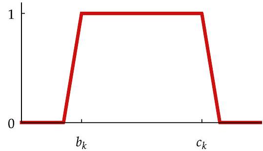
The graph of a continuous function g_{k} such that \left\|\chi_{\left[b_{k}, c_{k}\right]}-g_{k}\right\|_{1} is small.

EXERCISES 3B

1 Give an example of a sequence f_{1}, f_{2}, \ldots of functions from $\mathbf{Z}^{+}$to [0, \infty) such that

\lim {k \rightarrow \infty} f{k}(m)=0

for every $m \in \mathbf{Z}^{+}$but \lim _{k \rightarrow \infty} \int f_{k} d \mu=1, where \mu is counting measure on \mathbf{Z}^{+}.

2 Give an example of a sequence f_{1}, f_{2}, \ldots of continuous functions from \mathbf{R} to [0,1] such that

\lim {k \rightarrow \infty} f{k}(x)=0

for every x \in \mathbf{R} but \lim _{k \rightarrow \infty} \int f_{k} d \lambda=\infty, where \lambda is Lebesgue measure on \mathbf{R}.

3 Suppose \lambda is Lebesgue measure on \mathbf{R} and f: \mathbf{R} \rightarrow \mathbf{R} is a Borel measurable function such that \int|f| d \lambda<\infty. Define g: \mathbf{R} \rightarrow \mathbf{R} by

g(x)=\int_{(-\infty, x)} f d \lambda

Prove that g is uniformly continuous on \mathbf{R}.

4 (a) Suppose (X, \mathcal{S}, \mu) is a measure space with \mu(X)<\infty. Suppose that f: X \rightarrow[0, \infty) is a bounded $\mathcal{S}$-measurable function. Prove that

\int f d \mu=\inf \left{\sum_{j=1}^{m} \mu\left(A_{j}\right) \sup {A{j}} f: A_{1}, \ldots, A_{m} \text { is an } \mathcal{S} \text {-partition of } X\right}

(b) Show that the conclusion of part (a) can fail if the hypothesis that f is bounded is replaced by the hypothesis that \int f d \mu<\infty.

(c) Show that the conclusion of part (a) can fail if the condition that \mu(X)<\infty is deleted.

[Part (a) of this exercise shows that if we had defined an upper Lebesgue sum, then we could have used it to define the integral. However, parts (b) and (c) show that the hypotheses that f is bounded and that \mu(X)<\infty would be needed if defining the integral via the equation above. The definition of the integral via the lower Lebesgue sum does not require these hypotheses, showing the advantage of using the approach via the lower Lebesgue sum.]

5 Let \lambda denote Lebesgue measure on \mathbf{R}. Suppose f: \mathbf{R} \rightarrow \mathbf{R} is a Borel measurable function such that \int|f| d \lambda<\infty. Prove that

\lim {k \rightarrow \infty} \int{[-k, k]} f d \lambda=\int f d \lambda .

6 Let \lambda denote Lebesgue measure on \mathbf{R}. Give an example of a continuous function f:[0, \infty) \rightarrow \mathbf{R} such that \lim _{t \rightarrow \infty} \int_{[0, t]} f d \lambda exists (in \mathbf{R} ) but \int_{[0, \infty)} f d \lambda is not defined.

7 Let \lambda denote Lebesgue measure on \mathbf{R}. Give an example of a continuous function f:(0,1) \rightarrow \mathbf{R} such that \lim _{n \rightarrow \infty} \int_{\left(\frac{1}{n}, 1\right)} f d \lambda exists (in \mathbf{R} ) but \int_{(0,1)} f d \lambda is not defined.

8 Verify the assertion in 3.38.

9 Verify the assertion in Example 3.41.

10 (a) Suppose (X, \mathcal{S}, \mu) is a measure space such that \mu(X)<\infty. Suppose p, r are positive numbers with p<r. Prove that if f: X \rightarrow[0, \infty) is an $\mathcal{S}$-measurable function such that \int f^{r} d \mu<\infty, then \int f^{p} d \mu<\infty.

(b) Give an example to show that the result in part (a) can be false without the hypothesis that \mu(X)<\infty.

11 Suppose (X, \mathcal{S}, \mu) is a measure space and f \in \mathcal{L}^{1}(\mu). Prove that

{x \in X: f(x) \neq 0}

is the countable union of sets with finite $\mu$-measure.

12 Suppose

f_{k}(x)=\frac{(1-x)^{k} \cos \frac{k}{x}}{\sqrt{x}}

Prove that \lim _{k \rightarrow \infty} \int_{0}^{1} f_{k}=0.

13 Give an example of a sequence of nonnegative Borel measurable functions f_{1}, f_{2}, \ldots on [0,1] such that both the following conditions hold:

• \lim _{k \rightarrow \infty} \int_{0}^{1} f_{k}=0;
• \sup f_{k}(x)=\infty for every $m \in \mathbf{Z}^{+}$and every x \in[0,1]. k \geq m

14 Let \lambda denote Lebesgue measure on \mathbf{R}.

(a) Let f(x)=1 / \sqrt{x}. Prove that \int_{[0,1]} f d \lambda=2.

(b) Let f(x)=1 /\left(1+x^{2}\right). Prove that \int_{\mathbf{R}} f d \lambda=\pi.

(c) Let f(x)=(\sin x) / x. Show that the integral \int_{(0, \infty)} f d \lambda is not defined but \lim _{t \rightarrow \infty} \int_{(0, t)} f d \lambda exists in \mathbf{R}.

15 Prove or give a counterexample: If G is an open subset of (0,1), then \chi_{G} is Riemann integrable on [0,1].

16 Suppose f \in \mathcal{L}^{1}(\mathbf{R}).

(a) For t \in \mathbf{R}, define f_{t}: \mathbf{R} \rightarrow \mathbf{R} by f_{t}(x)=f(x-t). Prove that \lim _{t \rightarrow 0}\left\|f-f_{t}\right\|_{1}=0.

(b) For t>0, define f_{t}: \mathbf{R} \rightarrow \mathbf{R} by f_{t}(x)=f(t x). Prove that \lim _{t \rightarrow 1}\left\|f-f_{t}\right\|_{1}=0.

Chapter 4

Differentiation

Does there exist a Lebesgue measurable set that fills up exactly half of each interval? To get a feeling for this question, consider the set E=\left[0, \frac{1}{8}\right] \cup\left[\frac{1}{4}, \frac{3}{8}\right] \cup\left[\frac{1}{2}, \frac{5}{8}\right] \cup\left[\frac{3}{4}, \frac{7}{8}\right]. This set E has the property that

|E \cap[0, b]|=\frac{b}{2}

for b=0, \frac{1}{4}, \frac{1}{2}, \frac{3}{4}, 1. Does there exist a Lebesgue measurable set E \subset[0,1], perhaps constructed in a fashion similar to the Cantor set, such that the equation above holds for all b \in[0,1] ?

In this chapter we see how to answer this question by considering differentiation issues. We begin by developing a powerful tool called the Hardy-Littlewood maximal inequality. This tool is used to prove an almost everywhere version of the Fundamental Theorem of Calculus. These results lead us to an important theorem about the density of Lebesgue measurable sets.

Trinity College at the University of Cambridge in England. G. H. Hardy (1877-1947) and John Littlewood (1885-1977) were students and later faculty members here. If you have not already done so, you should read Hardy's remarkable book A Mathematician's Apology (do not skip the fascinating Foreword by C. P. Snow) and see the movie The Man Who Knew Infinity, which focuses on Hardy, Littlewood, and Srinivasa Ramanujan (1887-1920).

CC-BY-SA Rafa Esteve

4A Hardy-Littlewood Maximal Function

Markov's Inequality

The following result, called Markov's inequality, has a sweet, short proof. We will make good use of this result later in this chapter (see the proof of 4.10). Markov's inequality also leads to Chebyshev's inequality (see Exercise 2 in this section).

4.1 Markov's inequality

Suppose (X, \mathcal{S}, \mu) is a measure space and h \in \mathcal{L}^{1}(\mu). Then

\mu({x \in X:|h(x)| \geq c}) \leq \frac{1}{c}|h|_{1}

for every c>0.

Proof Suppose c>0. Then

\begin{aligned} \mu({x \in X:|h(x)| \geq c}) & =\frac{1}{c} \int_{{x \in X:|h(x)| \geq c}} c d \mu \ & \leq \frac{1}{c} \int_{{x \in X:|h(x)| \geq c}}|h| d \mu \ & \leq \frac{1}{c}|h|_{1}, \end{aligned}

as desired.

St. Petersburg University along the Neva River in St. Petersburg, Russia. Andrei Markov (1856-1922) was a student and then a faculty member here. CC-BY-SA A. Savin

Vitali Covering Lemma

4.2 Definition 3 times a bounded nonempty open interval

Suppose I is a bounded nonempty open interval of \mathbf{R}. Then 3 * I denotes the open interval with the same center as I and three times the length of I.

4.3 Example 3 times an interval

If I=(0,10), then 3 * I=(-10,20).

The next result is a key tool in the proof of the Hardy-Littlewood maximal inequality (4.8).

4.4 Vitali Covering Lemma

Suppose I_{1}, \ldots, I_{n} is a list of bounded nonempty open intervals of \mathbf{R}. Then there exists a disjoint sublist I_{k_{1}}, \ldots, I_{k_{m}} such that

I_{1} \cup \cdots \cup I_{n} \subset\left(3 * I_{k_{1}}\right) \cup \cdots \cup\left(3 * I_{k_{m}}\right) .

4.5 Example Vitali Covering Lemma

Suppose n=4 and

I_{1}=(0,10), \quad I_{2}=(9,15), \quad I_{3}=(14,22), \quad I_{4}=(21,31) .

Then

3 * I_{1}=(-10,20), \quad 3 * I_{2}=(3,21), \quad 3 * I_{3}=(6,30), \quad 3 * I_{4}=(11,41) .

Thus

I_{1} \cup I_{2} \cup I_{3} \cup I_{4} \subset\left(3 * I_{1}\right) \cup\left(3 * I_{4}\right)

In this example, I_{1}, I_{4} is the only sublist of I_{1}, I_{2}, I_{3}, I_{4} that produces the conclusion of the Vitali Covering Lemma.

Proof of 4.4 Let k_{1} be such that

\left|I_{k_{1}}\right|=\max \left{\left|I_{1}\right|, \ldots,\left|I_{n}\right|\right}

Suppose k_{1}, \ldots, k_{j} have been chosen. Let k_{j+1} be such that \left|I_{k_{j+1}}\right| is as large as possible subject to the condition that I_{k_{1}}, \ldots, I_{k_{j+1}} are disjoint. If there is no choice of k_{j+1} such that I_{k_{1}}, \ldots, I_{k_{j+1}} are disjoint, then the procedure terminates.

The technique used here is called a greedy algorithm because at each stage we select the largest remaining interval that is disjoint from the previously selected intervals.

Because we start with a finite list, the procedure must eventually terminate after some number m of choices.

Suppose j \in\{1, \ldots, n\}. To complete the proof, we must show that

I_{j} \subset\left(3 * I_{k_{1}}\right) \cup \cdots \cup\left(3 * I_{k_{m}}\right)

If j \in\left\{k_{1}, \ldots, k_{m}\right\}, then the inclusion above obviously holds.

Thus assume that j \notin\left\{k_{1}, \ldots, k_{m}\right\}. Because the process terminated without selecting j, the interval I_{j} is not disjoint from all of I_{k_{1}}, \ldots, I_{k_{m}}. Let I_{k_{L}} be the first interval on this list not disjoint from I_{j}; thus I_{j} is disjoint from I_{k_{1}}, \ldots, I_{k_{L-1}}. Because j was not chosen in step L, we conclude that \left|I_{k_{L}}\right| \geq\left|I_{j}\right|. Because I_{k_{L}} \cap I_{j} \neq \varnothing, this last inequality implies (easy exercise) that I_{j} \subset 3 * I_{k_{L}}, completing the proof.

Hardy-Littlewood Maximal Inequality

Now we come to a brilliant definition that turns out to be extraordinarily useful.

4.6 Definition Hardy-Littlewood maximal function; h^{*}

Suppose h: \mathbf{R} \rightarrow \mathbf{R} is a Lebesgue measurable function. Then the HardyLittlewood maximal function of h is the function h^{*}: \mathbf{R} \rightarrow[0, \infty] defined by

h^{*}(b)=\sup {t>0} \frac{1}{2 t} \int{b-t}^{b+t}|h|

In other words, h^{*}(b) is the supremum over all bounded intervals centered at b of the average of |h| on those intervals.

4.7 Example Hardy-Littlewood maximal function of \chi_{[0,1]}

As usual, let \chi_{[0,1]} denote the characteristic function of the interval [0,1]. Then

\left(\chi_{[0,1]}\right)^{*}(b)= \begin{cases}\frac{1}{2(1-b)} & \text { if } b \leq 0 \ 1 & \text { if } 0<b<1 \ \frac{1}{2 b} & \text { if } b \geq 1\end{cases}

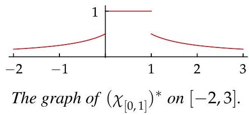
as you should verify.

If h: \mathbf{R} \rightarrow \mathbf{R} is Lebesgue measurable and c \in \mathbf{R}, then \left\{b \in \mathbf{R}: h^{*}(b)>c\right\} is an open subset of \mathbf{R}, as you are asked to prove in Exercise 9 in this section. Thus h^{*} is a Borel measurable function.

Suppose h \in \mathcal{L}^{1}(\mathbf{R}) and c>0. Markov's inequality (4.1) estimates the size of the set on which |h| is larger than c. Our next result estimates the size of the set on which h^{*} is larger than c. The Hardy-Littlewood maximal inequality proved in the next result is a key ingredient in the proof of the Lebesgue Differentiation Theorem (4.10). Note that this next result is considerably deeper than Markov's inequality.

4.8 Hardy-Littlewood maximal inequality

Suppose h \in \mathcal{L}^{1}(\mathbf{R}). Then

\left|\left{b \in \mathbf{R}: h^{*}(b)>c\right}\right| \leq \frac{3}{c}|h|_{1}

for every c>0.

Proof Suppose F is a closed bounded subset of \left\{b \in \mathbf{R}: h^{*}(b)>c\right\}. We will show that |F| \leq \frac{3}{c} \int_{-\infty}^{\infty}|h|, which implies our desired result [see Exercise 24(a) in Section 2D].

For each b \in F, there exists t_{b}>0 such that

\frac{1}{2 t_{b}} \int_{b-t_{b}}^{b+t_{b}}|h|>c

Clearly

F \subset \bigcup_{b \in F}\left(b-t_{b}, b+t_{b}\right) .

The Heine-Borel Theorem (2.12) tells us that this open cover of a closed bounded set has a finite subcover. In other words, there exist b_{1}, \ldots, b_{n} \in F such that

F \subset\left(b_{1}-t_{b_{1}}, b_{1}+t_{b_{1}}\right) \cup \cdots \cup\left(b_{n}-t_{b_{n}}, b_{n}+t_{b_{n}}\right) .

To make the notation cleaner, relabel the open intervals above as I_{1}, \ldots, I_{n}.

Now apply the Vitali Covering Lemma (4.4) to the list I_{1}, \ldots, I_{n}, producing a disjoint sublist I_{k_{1}}, \ldots, I_{k_{m}} such that

I_{1} \cup \cdots \cup I_{n} \subset\left(3 * I_{k_{1}}\right) \cup \cdots \cup\left(3 * I_{k_{m}}\right) .

Thus

\begin{aligned} |F| & \leq\left|I_{1} \cup \cdots \cup I_{n}\right| \ & \leq\left|\left(3 * I_{k_{1}}\right) \cup \cdots \cup\left(3 * I_{k_{m}}\right)\right| \ & \leq\left|3 * I_{k_{1}}\right|+\cdots+\left|3 * I_{k_{m}}\right| \ & =3\left(\left|I_{k_{1}}\right|+\cdots+\left|I_{k_{m}}\right|\right) \ & <\frac{3}{c}\left(\int_{I_{k_{1}}}|h|+\cdots+\int_{I_{k_{m}}}|h|\right) \ & \leq \frac{3}{c} \int_{-\infty}^{\infty}|h|, \end{aligned}

where the second-to-last inequality above comes from 4.9 (note that \left|I_{k_{j}}\right|=2 t_{b} for the choice of b corresponding to I_{k_{j}} ) and the last inequality holds because I_{k_{1}}, \ldots, I_{k_{m}} are disjoint.

The last inequality completes the proof.

EXERCISES 4A

1 Suppose (X, \mathcal{S}, \mu) is a measure space and h: X \rightarrow \mathbf{R} is an $\mathcal{S}$-measurable function. Prove that

\mu({x \in X:|h(x)| \geq c}) \leq \frac{1}{c^{p}} \int|h|^{p} d \mu

for all positive numbers c and p.

2 Suppose (X, \mathcal{S}, \mu) is a measure space with \mu(X)=1 and h \in \mathcal{L}^{1}(\mu). Prove that

\mu\left(\left{x \in X:\left|h(x)-\int h d \mu\right| \geq c\right}\right) \leq \frac{1}{c^{2}}\left(\int h^{2} d \mu-\left(\int h d \mu\right)^{2}\right)

for all c>0.

[The result above is called Chebyshev's inequality; it plays an important role in probability theory. Pafnuty Chebyshev (1821-1894) was Markov's thesis advisor.]

3 Suppose (X, \mathcal{S}, \mu) is a measure space. Suppose h \in \mathcal{L}^{1}(\mu) and \|h\|_{1}>0. Prove that there is at most one number c \in(0, \infty) such that

\mu({x \in X:|h(x)| \geq c})=\frac{1}{c}|h|_{1} .

4 Show that the constant 3 in the Vitali Covering Lemma (4.4) cannot be replaced by a smaller positive constant.

5 Prove the assertion left as an exercise in the last sentence of the proof of the Vitali Covering Lemma (4.4).

6 Verify the formula in Example 4.7 for the Hardy-Littlewood maximal function of \chi_{[0,1]}.

7 Find a formula for the Hardy-Littlewood maximal function of the characteristic function of [0,1] \cup[2,3].

8 Find a formula for the Hardy-Littlewood maximal function of the function h: \mathbf{R} \rightarrow[0, \infty) defined by

h(x)= \begin{cases}x & \text { if } 0 \leq x \leq 1 \ 0 & \text { otherwise }\end{cases}

9 Suppose h: \mathbf{R} \rightarrow \mathbf{R} is Lebesgue measurable. Prove that

\left{b \in \mathbf{R}: h^{*}(b)>c\right}

is an open subset of \mathbf{R} for every c \in \mathbf{R}.

10 Prove or give a counterexample: If h: \mathbf{R} \rightarrow[0, \infty) is an increasing function, then h^{*} is an increasing function.

11 Give an example of a Borel measurable function h: \mathbf{R} \rightarrow[0, \infty) such that h^{*}(b)<\infty for all b \in \mathbf{R} but \sup \left\{h^{*}(b): b \in \mathbf{R}\right\}=\infty.

12 Show that \left|\left\{b \in \mathbf{R}: h^{*}(b)=\infty\right\}\right|=0 for every h \in \mathcal{L}^{1}(\mathbf{R}).

13 Show that there exists h \in \mathcal{L}^{1}(\mathbf{R}) such that h^{*}(b)=\infty for every b \in \mathbf{Q}.

14 Suppose h \in \mathcal{L}^{1}(\mathbf{R}). Prove that

\left|\left{b \in \mathbf{R}: h^{*}(b) \geq c\right}\right| \leq \frac{3}{c}|h|_{1}

for every c>0.

[This result slightly strengthens the Hardy-Littlewood maximal inequality (4.8) because the set on the left side above includes those b \in \mathbf{R} such that h^{*}(b)=c. A much deeper strengthening comes from replacing the constant 3 in the HardyLittlewood maximal inequality with a smaller constant. In 2003, Antonios Melas answered what had been an open question about the best constant. He proved that the smallest constant that can replace 3 in the Hardy-Littlewood maximal inequality is (11+\sqrt{61}) / 12 \approx 1.56752; see Annals of Mathematics 157 (2003), 647-688.]

4B Derivatives of Integrals

Lebesgue Differentiation Theorem

The next result states that the average amount by which a function in \mathcal{L}^{1}(\mathbf{R}) differs from its values is small almost everywhere on small intervals. The 2 in the denominator of the fraction in the result below could be deleted, but its presence makes the length of the interval of integration nicely match the denominator 2 t.

The next result is called the Lebesgue Differentiation Theorem, even though no derivative is in sight. However, we will soon see how another version of this result deals with derivatives. The hard work takes place in the proof of this first version.

4.10 Lebesgue Differentiation Theorem, first version

Suppose f \in \mathcal{L}^{1}(\mathbf{R}). Then

\lim {t \downarrow 0} \frac{1}{2 t} \int{b-t}^{b+t}|f-f(b)|=0

for almost every b \in \mathbf{R}.

Before getting to the formal proof of this first version of the Lebesgue Differentiation Theorem, we pause to provide some motivation for the proof. If b \in \mathbf{R} and t>0, then 3.25 gives the easy estimate

\frac{1}{2 t} \int_{b-t}^{b+t}|f-f(b)| \leq \sup {|f(x)-f(b)|:|x-b| \leq t}

If f is continuous at b, then the right side of this inequality has limit 0 as t \downarrow 0, proving 4.10 in the special case in which f is continuous on \mathbf{R}.

To prove the Lebesgue Differentiation Theorem, we will approximate an arbitrary function in \mathcal{L}^{1}(\mathbf{R}) by a continuous function (using 3.48). The previous paragraph shows that the continuous function has the desired behavior. We will use the HardyLittlewood maximal inequality (4.8) to show that the approximation produces approximately the desired behavior. Now we are ready for the formal details of the proof.

Proof of 4.10 Let \delta>0. By 3.48, for each $k \in \mathbf{Z}^{+}$there exists a continuous function h_{k}: \mathbf{R} \rightarrow \mathbf{R} such that

4.11

\left|f-h_{k}\right|_{1}<\frac{\delta}{k 2^{k}} .

Let

B_{k}=\left{b \in \mathbf{R}:\left|f(b)-h_{k}(b)\right| \leq \frac{1}{k} \text { and }\left(f-h_{k}\right)^{*}(b) \leq \frac{1}{k}\right} \text {. }

Then

4.12 \mathbf{R} \backslash B_{k}=\left\{b \in \mathbf{R}:\left|f(b)-h_{k}(b)\right|>\frac{1}{k}\right\} \cup\left\{b \in \mathbf{R}:\left(f-h_{k}\right)^{*}(b)>\frac{1}{k}\right\}.

Markov's inequality (4.1) as applied to the function f-h_{k} and 4.11 imply that

4.13

\left|\left{b \in \mathbf{R}:\left|f(b)-h_{k}(b)\right|>\frac{1}{k}\right}\right|<\frac{\delta}{2^{k}}

The Hardy-Littlewood maximal inequality (4.8) as applied to the function f-h_{k} and 4.11 imply that

4.14

\left|\left{b \in \mathbf{R}:\left(f-h_{k}\right)^{*}(b)>\frac{1}{k}\right}\right|<\frac{3 \delta}{2^{k}} .

Now 4.12, 4.13, and 4.14 imply that

\left|\mathbf{R} \backslash B_{k}\right|<\frac{\delta}{2^{k-2}}

Let

B=\bigcap_{k=1}^{\infty} B_{k}

Then

4.15

|\mathbf{R} \backslash B|=\left|\bigcup_{k=1}^{\infty}\left(\mathbf{R} \backslash B_{k}\right)\right| \leq \sum_{k=1}^{\infty}\left|\mathbf{R} \backslash B_{k}\right|<\sum_{k=1}^{\infty} \frac{\delta}{2^{k-2}}=4 \delta

Suppose b \in B and t>0. Then for each $k \in \mathbf{Z}^{+}$we have

\begin{aligned} \frac{1}{2 t} \int_{b-t}^{b+t}|f-f(b)| & \leq \frac{1}{2 t} \int_{b-t}^{b+t}\left(\left|f-h_{k}\right|+\left|h_{k}-h_{k}(b)\right|+\left|h_{k}(b)-f(b)\right|\right) \ & \leq\left(f-h_{k}\right)^{*}(b)+\left(\frac{1}{2 t} \int_{b-t}^{b+t}\left|h_{k}-h_{k}(b)\right|\right)+\left|h_{k}(b)-f(b)\right| \ & \leq \frac{2}{k}+\frac{1}{2 t} \int_{b-t}^{b+t}\left|h_{k}-h_{k}(b)\right| . \end{aligned}

Because h_{k} is continuous, the last term is less than \frac{1}{k} for all t>0 sufficiently close to 0 (how close is sufficiently close depends upon k ). In other words, for each k \in \mathbf{Z}^{+}, we have

\frac{1}{2 t} \int_{b-t}^{b+t}|f-f(b)|<\frac{3}{k}

for all t>0 sufficiently close to 0 .

Hence we conclude that

\lim {t \downarrow 0} \frac{1}{2 t} \int{b-t}^{b+t}|f-f(b)|=0

for all b \in B.

Let A denote the set of numbers a \in \mathbf{R} such that

\lim {t \downarrow 0} \frac{1}{2 t} \int{a-t}^{a+t}|f-f(a)|

either does not exist or is nonzero. We have shown that A \subset(\mathbf{R} \backslash B). Thus

|A| \leq|\mathbf{R} \backslash B|<4 \delta

where the last inequality comes from 4.15 . Because \delta is an arbitrary positive number, the last inequality implies that |A|=0, completing the proof.

Derivatives

You should remember the following definition from your calculus course.

4.16 Definition derivative; g^{\prime}; differentiable

Suppose g: I \rightarrow \mathbf{R} is a function defined on an open interval I of \mathbf{R} and b \in I. The derivative of g at b, denoted g^{\prime}(b), is defined by

g^{\prime}(b)=\lim _{t \rightarrow 0} \frac{g(b+t)-g(b)}{t}

if the limit above exists, in which case g is called differentiable at b.

We now turn to the Fundamental Theorem of Calculus and a powerful extension that avoids continuity. These results show that differentiation and integration can be thought of as inverse operations.

You saw the next result in your calculus class, except now the function f is only required to be Lebesgue measurable (and its absolute value must have a finite Lebesgue integral). Of course, we also need to require f to be continuous at the crucial point b in the next result, because changing the value of f at a single number would not change the function g.

4.17 Fundamental Theorem of Calculus

Suppose f \in \mathcal{L}^{1}(\mathbf{R}). Define g: \mathbf{R} \rightarrow \mathbf{R} by

g(x)=\int_{-\infty}^{x} f

Suppose b \in \mathbf{R} and f is continuous at b. Then g is differentiable at b and

g^{\prime}(b)=f(b)

Proof If t \neq 0, then

\begin{aligned} \left|\frac{g(b+t)-g(b)}{t}-f(b)\right| & =\left|\frac{\int_{-\infty}^{b+t} f-\int_{-\infty}^{b} f}{t}-f(b)\right| \ & =\left|\frac{\int_{b}^{b+t} f}{t}-f(b)\right| \ & =\left|\frac{\int_{b}^{b+t}(f-f(b))}{t}\right| \ & \leq \sup _{{x \in \mathbf{R}:|x-b|<|t|}}|f(x)-f(b)| . \end{aligned}

If \varepsilon>0, then by the continuity of f at b, the last quantity is less than \varepsilon for t sufficiently close to 0 . Thus g is differentiable at b and g^{\prime}(b)=f(b).

A function in \mathcal{L}^{1}(\mathbf{R}) need not be continuous anywhere. Thus the Fundamental Theorem of Calculus (4.17) might provide no information about differentiating the integral of such a function. However, our next result states that all is well almost everywhere, even in the absence of any continuity of the function being integrated.

4.19 Lebesgue Differentiation Theorem, second version

Suppose f \in \mathcal{L}^{1}(\mathbf{R}). Define g: \mathbf{R} \rightarrow \mathbf{R} by

g(x)=\int_{-\infty}^{x} f

Then g^{\prime}(b)=f(b) for almost every b \in \mathbf{R}.

Proof Suppose t \neq 0. Then from 4.18 we have

\begin{aligned} \left|\frac{g(b+t)-g(b)}{t}-f(b)\right| & =\left|\frac{\int_{b}^{b+t}(f-f(b))}{t}\right| \ & \leq \frac{1}{t} \int_{b}^{b+t}|f-f(b)| \ & \leq \frac{1}{t} \int_{b-t}^{b+t}|f-f(b)| \end{aligned}

for all b \in \mathbf{R}. By the first version of the Lebesgue Differentiation Theorem (4.10), the last quantity has limit 0 as t \rightarrow 0 for almost every b \in \mathbf{R}. Thus g^{\prime}(b)=f(b) for almost every b \in \mathbf{R}.

Now we can answer the question raised on the opening page of this chapter.

4.20 no set constitutes exactly half of each interval

There does not exist a Lebesgue measurable set E \subset[0,1] such that

|E \cap[0, b]|=\frac{b}{2}

for all b \in[0,1]

Proof Suppose there does exist a Lebesgue measurable set E \subset[0,1] with the property above. Define g: \mathbf{R} \rightarrow \mathbf{R} by

g(b)=\int_{-\infty}^{b} \chi_{E} .

Thus g(b)=\frac{b}{2} for all b \in[0,1]. Hence g^{\prime}(b)=\frac{1}{2} for all b \in(0,1).

The Lebesgue Differentiation Theorem (4.19) implies that g^{\prime}(b)=\chi_{E}(b) for almost every b \in \mathbf{R}. However, \chi_{E} never takes on the value \frac{1}{2}, which contradicts the conclusion of the previous paragraph. This contradiction completes the proof.

The next result says that a function in \mathcal{L}^{1}(\mathbf{R}) is equal almost everywhere to the limit of its average over small intervals. These two-sided results generalize more naturally to higher dimensions (take the average over balls centered at b ) than the one-sided results.

4.21 \mathcal{L}^{1}(\mathbf{R}) function equals its local average almost everywhere

Suppose f \in \mathcal{L}^{1}(\mathbf{R}). Then

f(b)=\lim {t \downarrow 0} \frac{1}{2 t} \int{b-t}^{b+t} f

for almost every b \in \mathbf{R}.

Proof Suppose t>0. Then

\begin{aligned} \left|\left(\frac{1}{2 t} \int_{b-t}^{b+t} f\right)-f(b)\right| & =\left|\frac{1}{2 t} \int_{b-t}^{b+t}(f-f(b))\right| \ & \leq \frac{1}{2 t} \int_{b-t}^{b+t}|f-f(b)| . \end{aligned}

The desired result now follows from the first version of the Lebesgue Differentiation Theorem (4.10).

Again, the conclusion of the result above holds at every number b at which f is continuous. The remarkable part of the result above is that even if f is discontinuous everywhere, the conclusion holds for almost every real number b.

Density

The next definition captures the notion of the proportion of a set in small intervals centered at a number b.

4.22 Definition density

Suppose E \subset \mathbf{R}. The density of E at a number b \in \mathbf{R} is

\lim _{t \downarrow 0} \frac{|E \cap(b-t, b+t)|}{2 t}

if this limit exists (otherwise the density of E at b is undefined).

4.23 Example density of an interval

The density of [0,1] at b= \begin{cases}1 & \text { if } b \in(0,1), \\ \frac{1}{2} & \text { if } b=0 \text { or } b=1 \\ 0 & \text { otherwise. }\end{cases}

The next beautiful result shows the power of the techniques developed in this chapter.

4.24 Lebesgue Density Theorem

Suppose E \subset \mathbf{R} is a Lebesgue measurable set. Then the density of E is 1 at almost every element of E and is 0 at almost every element of \mathbf{R} \backslash E.

Proof First suppose |E|<\infty. Thus \chi_{E} \in \mathcal{L}^{1}(\mathbf{R}). Because

\frac{|E \cap(b-t, b+t)|}{2 t}=\frac{1}{2 t} \int_{b-t}^{b+t} \chi_{E}

for every t>0 and every b \in \mathbf{R}, the desired result follows immediately from 4.21.

Now consider the case where |E|=\infty [which means that \chi_{E} \notin \mathcal{L}^{1}(\mathbf{R}) and hence 4.21 as stated cannot be used]. For k \in \mathbf{Z}^{+}, let E_{k}=E \cap(-k, k). If |b|<k, then the density of E at b equals the density of E_{k} at b. By the previous paragraph as applied to E_{k}, there are sets F_{k} \subset E_{k} and G_{k} \subset \mathbf{R} \backslash E_{k} such that \left|F_{k}\right|=\left|G_{k}\right|=0 and the density of E_{k} equals 1 at every element of E_{k} \backslash F_{k} and the density of E_{k} equals 0 at every element of \left(\mathbf{R} \backslash E_{k}\right) \backslash G_{k}.

Let F=\bigcup_{k=1}^{\infty} F_{k} and G=\bigcup_{k=1}^{\infty} G_{k}. Then |F|=|G|=0 and the density of E is 1 at every element of E \backslash F and is 0 at every element of (\mathbf{R} \backslash E) \backslash G.

The bad Borel set provided by the next result leads to a bad Borel measurable function. Specifically, let E be the bad Borel set in 4.25. Then \chi_{E} is a Borel measurable function that is discontinuous everywhere. Furthermore, the function \chi_{E} cannot be modified on a set of measure 0 to be continuous anywhere (in contrast to the function \chi_{\mathbf{Q}} ).

The Lebesgue Density Theorem makes the example provided by the next result somewhat surprising. Be sure to spend some time pondering why the next result does not contradict the Lebesgue Density Theorem. Also, compare the next result to 4.20.

Even though the function \chi_{E} discussed in the paragraph above is continuous nowhere and every modification of this function on a set of measure 0 is also continuous nowhere, the function g defined by

g(b)=\int_{0}^{b} \chi_{E}

is differentiable almost everywhere (by 4.19).

The proof of 4.25 given below is based on an idea of Walter Rudin.

4.25 bad Borel set

There exists a Borel set E \subset \mathbf{R} such that

0<|E \cap I|<|I|

for every nonempty bounded open interval I.

Proof We use the following fact in our construction:

4.26 Suppose G is a nonempty open subset of \mathbf{R}. Then there exists a closed set F \subset G \backslash Q such that |F|>0.

To prove 4.26, let J be a closed interval contained in G such that 0<|J|. Let r_{1}, r_{2}, \ldots be a list of all the rational numbers. Let

F=J \backslash \bigcup_{k=1}^{\infty}\left(r_{k}-\frac{|J|}{2^{k+2}}, r_{k}+\frac{|J|}{2^{k+2}}\right)

Then F is a closed subset of \mathbf{R} and F \subset J \backslash \mathbf{Q} \subset G \backslash \mathbf{Q}. Also, |J \backslash F| \leq \frac{1}{2}|J| because J \backslash F \subset \bigcup_{k=1}^{\infty}\left(r_{k}-\frac{|J|}{2^{k+2}}, r_{k}+\frac{|J|}{2^{k+2}}\right). Thus

|F|=|J|-|J \backslash F| \geq \frac{1}{2}|J|>0

completing the proof of 4.26 .

To construct the set E with the desired properties, let I_{1}, I_{2}, \ldots be a sequence consisting of all nonempty bounded open intervals of \mathbf{R} with rational endpoints. Let F_{0}=\widehat{F}_{0}=\varnothing, and inductively construct sequences F_{1}, F_{2}, \ldots and \widehat{F}_{1}, \widehat{F}_{2}, \ldots of closed subsets of \mathbf{R} as follows: Suppose $n \in \mathbf{Z}^{+}$and F_{0}, \ldots, F_{n-1} and \widehat{F}_{0}, \ldots, \widehat{F}_{n-1} have been chosen as closed sets that contain no rational numbers. Thus

I_{n} \backslash\left(\widehat{F_{0}} \cup \ldots \cup \widehat{F}_{n-1}\right)

is a nonempty open set (nonempty because it contains all rational numbers in I_{n} ). Applying 4.26 to the open set above, we see that there is a closed set F_{n} contained in the set above such that F_{n} contains no rational numbers and \left|F_{n}\right|>0. Applying 4.26 again, but this time to the open set

I_{n} \backslash\left(F_{0} \cup \ldots \cup F_{n}\right)

which is nonempty because it contains all rational numbers in I_{n}, we see that there is a closed set \widehat{F}_{n} contained in the set above such that \widehat{F}_{n} contains no rational numbers and \left|\widehat{F}_{n}\right|>0.

Now let

E=\bigcup_{k=1}^{\infty} F_{k}

Our construction implies that F_{k} \cap \widehat{F}_{n}=\varnothing for all k, n \in \mathbf{Z}^{+}. Thus E \cap \widehat{F}_{n}=\varnothing for all n \in \mathbf{Z}^{+}. Hence \widehat{F}_{n} \subset I_{n} \backslash E for all n \in \mathbf{Z}^{+}.

Suppose I is a nonempty bounded open interval. Then I_{n} \subset I for some n \in \mathbf{Z}^{+}. Thus

0<\left|F_{n}\right| \leq\left|E \cap I_{n}\right| \leq|E \cap I|

Also,

|E \cap I|=|I|-|I \backslash E| \leq|I|-\left|I_{n} \backslash E\right| \leq|I|-\left|\widehat{F}_{n}\right|<|I|,

completing the proof.

EXERCISES 4B

For f \in \mathcal{L}^{1}(\mathrm{R}) and I an interval of \mathrm{R} with 0<|I|<\infty, let f_{I} denote the average of f on I. In other words, f_{I}=\frac{1}{|I|} \int_{I} f.

1 Suppose f \in \mathcal{L}^{1}(\mathbf{R}). Prove that

\lim {t \downarrow 0} \frac{1}{2 t} \int{b-t}^{b+t}\left|f-f_{[b-t, b+t]}\right|=0

for almost every b \in \mathbf{R}.

2 Suppose f \in \mathcal{L}^{1}(\mathbf{R}). Prove that

\lim {t \downarrow 0} \sup \left{\frac{1}{|I|} \int{I}\left|f-f_{I}\right|: I \text { is an interval of length } t \text { containing } b\right}=0

for almost every b \in \mathbf{R}.

3 Suppose f: \mathbf{R} \rightarrow \mathbf{R} is a Lebesgue measurable function such that f^{2} \in \mathcal{L}^{1}(\mathbf{R}). Prove that

\lim {t \downarrow 0} \frac{1}{2 t} \int{b-t}^{b+t}|f-f(b)|^{2}=0

for almost every b \in \mathbf{R}.

4 Prove that the Lebesgue Differentiation Theorem (4.19) still holds if the hypothesis that \int_{-\infty}^{\infty}|f|<\infty is weakened to the requirement that \int_{-\infty}^{x}|f|<\infty for all x \in \mathbf{R}.

5 Suppose f: \mathbf{R} \rightarrow \mathbf{R} is a Lebesgue measurable function. Prove that

|f(b)| \leq f^{*}(b)

for almost every b \in \mathbf{R}.

6 Prove that if h \in \mathcal{L}^{1}(\mathbf{R}) and \int_{-\infty}^{s} h=0 for all s \in \mathbf{R}, then h(s)=0 for almost every s \in \mathbf{R}.

7 Give an example of a Borel subset of \mathbf{R} whose density at 0 is not defined.

8 Give an example of a Borel subset of \mathbf{R} whose density at 0 is \frac{1}{3}.

9 Prove that if t \in[0,1], then there exists a Borel set E \subset \mathbf{R} such that the density of E at 0 is t.

10 Suppose E is a Lebesgue measurable subset of \mathbf{R} such that the density of E equals 1 at every element of E and equals 0 at every element of \mathbf{R} \backslash E. Prove that E=\varnothing or E=\mathbf{R}.

Chapter 5

Product Measures

Lebesgue measure on \mathbf{R} generalizes the notion of the length of an interval. In this chapter, we see how two-dimensional Lebesgue measure on \mathbf{R}^{2} generalizes the notion of the area of a rectangle. More generally, we construct new measures that are the products of two measures.

Once these new measures have been constructed, the question arises of how to compute integrals with respect to these new measures. Beautiful theorems proved in the first decade of the twentieth century allow us to compute integrals with respect to product measures as iterated integrals involving the two measures that produced the product. Furthermore, we will see that under reasonable conditions we can switch the order of an iterated integral.

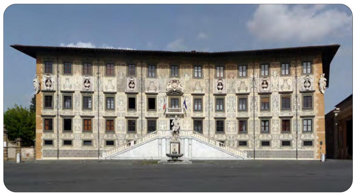
Main building of Scuola Normale Superiore di Pisa, the university in Pisa, Italy, where Guido Fubini (1879-1943) received his PhD in 1900. In 1907 Fubini proved that under reasonable conditions, an integral with respect to a product measure can be computed as an iterated integral and that the order of integration can be switched. Leonida Tonelli (1885-1943) also taught for many years in Pisa; he also proved a crucial theorem about interchanging the order of integration in an iterated integral. CC-BY-SA Lucarelli

5A Products of Measure Spaces

Products of $\sigma$-Algebras

Our first step in constructing product measures is to construct the product of two $\sigma$-algebras. We begin with the following definition.

5.1 Definition rectangle

Suppose X and Y are sets. A rectangle in X \times Y is a set of the form A \times B, where A \subset X and B \subset Y.

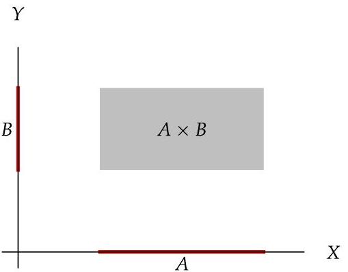
Now we can define the product of two $\sigma$-algebras.

5.2 Definition product of two $\sigma$-algebras; \mathcal{S} \otimes \mathcal{T}; measurable rectangle

Suppose (X, \mathcal{S}) and (Y, \mathcal{T}) are measurable spaces. Then

• the product \mathcal{S} \otimes \mathcal{T} is defined to be the smallest $\sigma$-algebra on X \times Y that contains

{A \times B: A \in \mathcal{S}, B \in \mathcal{T}}

• a measurable rectangle in \mathcal{S} \otimes \mathcal{T} is a set of the form A \times B, where A \in \mathcal{S} and B \in \mathcal{T}.

Using the terminology introduced in the second bullet point above, we can say that \mathcal{S} \otimes \mathcal{T} is the smallest $\sigma$-algebra containing all the measurable rectangles in \mathcal{S} \otimes \mathcal{T}. Exercise 1 in this section asks you to show that the measurable rectangles in \mathcal{S} \otimes \mathcal{T} are the only rectangles in

The notation \mathcal{S} \times \mathcal{T} is not used because \mathcal{S} and \mathcal{T} are sets (of sets), and thus the notation \mathcal{S} \times \mathcal{T} already is defined to mean the set of all ordered pairs of the form (A, B), where A \in \mathcal{S} and B \in \mathcal{T}. X \times Y that are in \mathcal{S} \otimes \mathcal{T}.

The notion of cross sections plays a crucial role in our development of product measures. First, we define cross sections of sets, and then we define cross sections of functions.

5.3 Definition cross sections of sets; [E]_{a} and [E]^{b}

Suppose X and Y are sets and E \subset X \times Y. Then for a \in X and b \in Y, the cross sections [E]_{a} and [E]^{b} are defined by

[E]_{a}={y \in Y:(a, y) \in E} \quad \text { and } \quad[E]^{b}={x \in X:(x, b) \in E}

5.4 Example cross sections of a subset of X \times Y

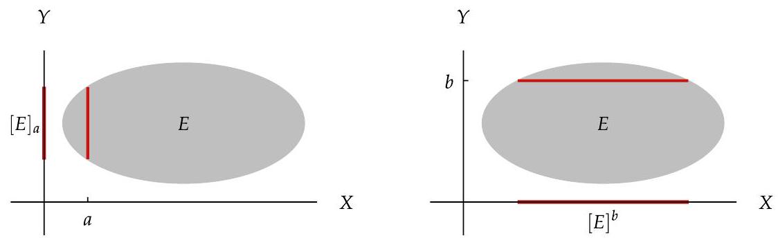
5.5 Example cross sections of rectangles

Suppose X and Y are sets and A \subset X and B \subset Y. If a \in X and b \in Y, then

[A \times B]_{a}=\left{\begin{array}{ll} B & \text { if } a \in A, \ \varnothing & \text { if } a \notin A \end{array} \quad \text { and } \quad[A \times B]^{b}= \begin{cases}A & \text { if } b \in B \ \varnothing & \text { if } b \notin B\end{cases}\right.

as you should verify.

The next result shows that cross sections preserve measurability.

5.6 cross sections of measurable sets are measurable

Suppose \mathcal{S} is a $\sigma$-algebra on X and \mathcal{T} is a $\sigma$-algebra on Y. If E \in \mathcal{S} \otimes \mathcal{T}, then

[E]_{a} \in \mathcal{T} \text { for every } a \in X \quad \text { and } \quad[E]^{b} \in \mathcal{S} \text { for every } b \in Y

Proof Let \mathcal{E} denote the collection of subsets E of X \times Y for which the conclusion of this result holds. Then A \times B \in \mathcal{E} for all A \in \mathcal{S} and all B \in \mathcal{T} (by Example 5.5).

The collection \mathcal{E} is closed under complementation and countable unions because

[(X \times Y) \backslash E]{a}=Y \backslash[E]{a}

and

\left[E_{1} \cup E_{2} \cup \cdots\right]{a}=\left[E{1}\right]{a} \cup\left[E{2}\right]_{a} \cup \cdots

for all subsets E, E_{1}, E_{2}, \ldots of X \times Y and all a \in X, as you should verify, with similar statements holding for cross sections with respect to all b \in Y.

Because \mathcal{E} is a $\sigma$-algebra containing all the measurable rectangles in \mathcal{S} \otimes \mathcal{T}, we conclude that \mathcal{E} contains \mathcal{S} \otimes \mathcal{T}.

Now we define cross sections of functions.

5.7 Definition cross sections of functions; [f]_{a} and [f]^{b}

Suppose X and Y are sets and f: X \times Y \rightarrow \mathbf{R} is a function. Then for a \in X and b \in Y, the cross section functions [f]_{a}: Y \rightarrow \mathbf{R} and [f]^{b}: X \rightarrow \mathbf{R} are defined by

[f]_{a}(y)=f(a, y) \text { for } y \in Y \quad \text { and }[f]^{b}(x)=f(x, b) \text { for } x \in X

5.8 Example cross sections

• Suppose f: \mathbf{R} \times \mathbf{R} \rightarrow \mathbf{R} is defined by f(x, y)=5 x^{2}+y^{3}. Then

[f]_{2}(y)=20+y^{3} \text { and }[f]^{3}(x)=5 x^{2}+27

for all y \in \mathbf{R} and all x \in \mathbf{R}, as you should verify.

• Suppose X and Y are sets and A \subset X and B \subset Y. If a \in X and b \in Y, then

\left[\chi_{A \times B}\right]{a}=\chi{A}(a) \chi_{B} \quad \text { and } \quad\left[\chi_{A \times B}\right]^{b}=\chi_{B}(b) \chi_{A} \text {, }

as you should verify.

The next result shows that cross sections preserve measurability, this time in the context of functions rather than sets.

5.9 cross sections of measurable functions are measurable

Suppose \mathcal{S} is a $\sigma$-algebra on X and \mathcal{T} is a $\sigma$-algebra on Y. Suppose f: X \times Y \rightarrow \mathbf{R} is an $\mathcal{S} \otimes \mathcal{T}$-measurable function. Then

[f]_{a} is a $\mathcal{T}$-measurable function on Y for every a \in X

and

[f]^{b} \text { is an } \mathcal{S} \text {-measurable function on } X \text { for every } b \in Y \text {. }

Proof Suppose D is a Borel subset of \mathbf{R} and a \in X. If y \in Y, then

\begin{aligned} y \in\left([f]{a}\right)^{-1}(D) & \Longleftrightarrow[f]{a}(y) \in D \ & \Longleftrightarrow f(a, y) \in D \ & \Longleftrightarrow(a, y) \in f^{-1}(D) \ & \Longleftrightarrow y \in\left[f^{-1}(D)\right]_{a} . \end{aligned}

Thus

\left([f]{a}\right)^{-1}(D)=\left[f^{-1}(D)\right]{a} .

Because f is an $\mathcal{S} \otimes \mathcal{T}$-measurable function, f^{-1}(D) \in \mathcal{S} \otimes \mathcal{T}. Thus the equation above and 5.6 \mathrm{imply} that \left([f]_{a}\right)^{-1}(D) \in \mathcal{T}. Hence [f]_{a} is a $\mathcal{T}$-measurable function.

The same ideas show that [f]^{b} is an $\mathcal{S}$-measurable function for every b \in Y.

Monotone Class Theorem

The following standard two-step technique often works to prove that every set in a $\sigma$-algebra has a certain property:

1. show that every set in a collection of sets that generates the $\sigma$-algebra has the property;
2. show that the collection of sets that has the property is a $\sigma$-algebra.

For example, the proof of 5.6 used the technique above-first we showed that every measurable rectangle in \mathcal{S} \otimes \mathcal{T} has the desired property, then we showed that the collection of sets that has the desired property is a $\sigma$-algebra (this completed the proof because \mathcal{S} \otimes \mathcal{T} is the smallest $\sigma$-algebra containing the measurable rectangles).

The technique outlined above should be used when possible. However, in some situations there seems to be no reasonable way to verify that the collection of sets with the desired property is a $\sigma$-algebra. We will encounter this situation in the next subsection. To deal with it, we need to introduce another technique that involves what are called monotone classes.

The following definition will be used in our main theorem about monotone classes.

5.10 Definition algebra

Suppose W is a set and \mathcal{A} is a set of subsets of W. Then \mathcal{A} is called an algebra on W if the following three conditions are satisfied:

• \varnothing \in \mathcal{A};
• if E \in \mathcal{A}, then W \backslash E \in \mathcal{A};
• if E and F are elements of \mathcal{A}, then E \cup F \in \mathcal{A}.

Thus an algebra is closed under complementation and under finite unions; a $\sigma$-algebra is closed under complementation and countable unions.

5.11 Example collection of finite unions of intervals is an algebra

Suppose \mathcal{A} is the collection of all finite unions of intervals of \mathbf{R}. Here we are including all intervals - open intervals, closed intervals, bounded intervals, unbounded intervals, sets consisting of only a single point, and intervals that are neither open nor closed because they contain one endpoint but not the other endpoint.

Clearly \mathcal{A} is closed under finite unions. You should also verify that \mathcal{A} is closed under complementation. Thus \mathcal{A} is an algebra on \mathbf{R}.

5.12 Example collection of countable unions of intervals is not an algebra

Suppose \mathcal{A} is the collection of all countable unions of intervals of \mathbf{R}.

Clearly \mathcal{A} is closed under finite unions (and also under countable unions). You should verify that \mathcal{A} is not closed under complementation. Thus \mathcal{A} is neither an algebra nor a $\sigma$-algebra on \mathbf{R}.

The following result provides an example of an algebra that we will exploit.

5.13 the set of finite unions of measurable rectangles is an algebra

Suppose (X, \mathcal{S}) and (Y, \mathcal{T}) are measurable spaces. Then

(a) the set of finite unions of measurable rectangles in \mathcal{S} \otimes \mathcal{T} is an algebra on X \times Y;

(b) every finite union of measurable rectangles in \mathcal{S} \otimes \mathcal{T} can be written as a finite union of disjoint measurable rectangles in \mathcal{S} \otimes \mathcal{T}.

Proof Let \mathcal{A} denote the set of finite unions of measurable rectangles in \mathcal{S} \otimes \mathcal{T}. Obviously \mathcal{A} is closed under finite unions.

The collection \mathcal{A} is also closed under finite intersections. To verify this claim, note that if A_{1}, \ldots, A_{n}, C_{1}, \ldots, C_{m} \in \mathcal{S} and B_{1}, \ldots, B_{n}, D_{1}, \ldots, D_{m} \in \mathcal{T}, then

\begin{aligned} & \left(\left(A_{1} \times B_{1}\right) \cup \cdots \cup\left(A_{n} \times B_{n}\right)\right) \cap\left(\left(C_{1} \times D_{1}\right) \cup \cdots \cup\left(C_{m} \times D_{m}\right)\right) \ & =\bigcup_{j=1}^{n} \bigcup_{k=1}^{m}\left(\left(A_{j} \times B_{j}\right) \cap\left(C_{k} \times D_{k}\right)\right) \ & =\bigcup_{j=1}^{n} \bigcup_{k=1}^{m}\left(\left(A_{j} \cap C_{k}\right) \times\left(B_{j} \cap D_{k}\right)\right), \quad A \times B \end{aligned}

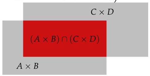
Intersection of two rectangles is a rectangle.

which implies that \mathcal{A} is closed under finite intersections.

If A \in \mathcal{S} and B \in \mathcal{T}, then

(X \times Y) \backslash(A \times B)=((X \backslash A) \times Y) \cup(X \times(Y \backslash B))

Hence the complement of each measurable rectangle in \mathcal{S} \otimes \mathcal{T} is in \mathcal{A}. Thus the complement of a finite union of measurable rectangles in \mathcal{S} \otimes \mathcal{T} is in \mathcal{A} (use De Morgan's Laws and the result in the previous paragraph that \mathcal{A} is closed under finite intersections). In other words, \mathcal{A} is closed under complementation, completing the proof of (a).

To prove (b), note that if A \times B and C \times D are measurable rectangles in \mathcal{S} \otimes \mathcal{T}, then (as can be verified in the figure above)

5.14(A \times B) \cup(C \times D)=(A \times B) \cup(C \times(D \backslash B)) \cup((C \backslash A) \times(B \cap D)) .

The equation above writes the union of two measurable rectangles in \mathcal{S} \otimes \mathcal{T} as the union of three disjoint measurable rectangles in \mathcal{S} \otimes \mathcal{T}.

Now consider any finite union of measurable rectangles in \mathcal{S} \otimes \mathcal{T}. If this is not a disjoint union, then choose any nondisjoint pair of measurable rectangles in the union and replace those two measurable rectangles with the union of three disjoint measurable rectangles as in 5.14. Iterate this process until obtaining a disjoint union of measurable rectangles.

Now we define a monotone class as a collection of sets that is closed under countable increasing unions and under countable decreasing intersections.

5.15 Definition monotone class

Suppose W is a set and \mathcal{M} is a set of subsets of W. Then \mathcal{M} is called a monotone class on W if the following two conditions are satisfied:

• If E_{1} \subset E_{2} \subset \cdots is an increasing sequence of sets in \mathcal{M}, then \bigcup_{k=1}^{\infty} E_{k} \in \mathcal{M};
• If E_{1} \supset E_{2} \supset \cdots is a decreasing sequence of sets in \mathcal{M}, then \bigcap_{k=1}^{\infty} E_{k} \in \mathcal{M}.

Clearly every $\sigma$-algebra is a monotone class. However, some monotone classes are not closed under even finite unions, as shown by the next example.

5.16 Example a monotone class that is not an algebra

Suppose \mathcal{A} is the collection of all intervals of \mathbf{R}. Then \mathcal{A} is closed under countable increasing unions and countable decreasing intersections. Thus \mathcal{A} is a monotone class on \mathbf{R}. However, \mathcal{A} is not closed under finite unions, and \mathcal{A} is not closed under complementation. Thus \mathcal{A} is neither an algebra nor a $\sigma$-algebra on \mathbf{R}.

If \mathcal{A} is a collection of subsets of some set W, then the intersection of all monotone classes on W that contain \mathcal{A} is a monotone class that contains \mathcal{A}. Thus this intersection is the smallest monotone class on W that contains \mathcal{A}.

The next result provides a useful tool when the standard technique for showing that every set in a $\sigma$-algebra has a certain property does not work.

5.17 Monotone Class Theorem

Suppose \mathcal{A} is an algebra on a set W. Then the smallest $\sigma$-algebra containing \mathcal{A} is the smallest monotone class containing \mathcal{A}.

Proof Let \mathcal{M} denote the smallest monotone class containing \mathcal{A}. Because every \sigma algebra is a monotone class, \mathcal{M} is contained in the smallest $\sigma$-algebra containing \mathcal{A}.

To prove the inclusion in the other direction, first suppose A \in \mathcal{A}. Let

\mathcal{E}={E \in \mathcal{M}: A \cup E \in \mathcal{M}}

Then \mathcal{A} \subset \mathcal{E} (because the union of two sets in \mathcal{A} is in \mathcal{A} ). A moment's thought shows that \mathcal{E} is a monotone class. Thus the smallest monotone class that contains \mathcal{A} is contained in \mathcal{E}, meaning that \mathcal{M} \subset \mathcal{E}. Hence we have proved that A \cup E \in \mathcal{M} for every E \in \mathcal{M}.

Now let

\mathcal{D}={D \in \mathcal{M}: D \cup E \in \mathcal{M} \text { for all } E \in \mathcal{M}}

The previous paragraph shows that \mathcal{A} \subset \mathcal{D}. A moment's thought again shows that \mathcal{D} is a monotone class. Thus, as in the previous paragraph, we conclude that \mathcal{M} \subset \mathcal{D}. Hence we have proved that D \cup E \in \mathcal{M} for all D, E \in \mathcal{M}.

The paragraph above shows that the monotone class \mathcal{M} is closed under finite unions. Now if E_{1}, E_{2}, \ldots \in \mathcal{M}, then

E_{1} \cup E_{2} \cup E_{3} \cup \cdots=E_{1} \cup\left(E_{1} \cup E_{2}\right) \cup\left(E_{1} \cup E_{2} \cup E_{3}\right) \cup \cdots,

which is an increasing union of a sequence of sets in \mathcal{M} (by the previous paragraph). We conclude that \mathcal{M} is closed under countable unions.

Finally, let

\mathcal{M}^{\prime}={E \in \mathcal{M}: W \backslash E \in \mathcal{M}}

Then \mathcal{A} \subset \mathcal{M}^{\prime} (because \mathcal{A} is closed under complementation). Once again, you should verify that \mathcal{M}^{\prime} is a monotone class. Thus \mathcal{M} \subset \mathcal{M}^{\prime}. We conclude that \mathcal{M} is closed under complementation.

The two previous paragraphs show that \mathcal{M} is closed under countable unions and under complementation. Thus \mathcal{M} is a $\sigma$-algebra that contains \mathcal{A}. Hence \mathcal{M} contains the smallest $\sigma$-algebra containing \mathcal{A}, completing the proof.

Products of Measures

The following definitions will be useful.

5.18 Definition finite measure; $\sigma$-finite measure

• A measure \mu on a measurable space (X, \mathcal{S}) is called finite if \mu(X)<\infty.
• A measure is called $\sigma$-finite if the whole space can be written as the countable union of sets with finite measure.
• More precisely, a measure \mu on a measurable space (X, \mathcal{S}) is called $\sigma$-finite if there exists a sequence X_{1}, X_{2}, \ldots of sets in \mathcal{S} such that

X=\bigcup_{k=1}^{\infty} X_{k} \quad \text { and } \quad \mu\left(X_{k}\right)<\infty \text { for every } k \in \mathbf{Z}^{+} \text {. }

5.19 Example finite and $\sigma$-finite measures

• Lebesgue measure on the interval [0,1] is a finite measure.
• Lebesgue measure on \mathbf{R} is not a finite measure but is a $\sigma$-finite measure.
• Counting measure on \mathbf{R} is not a $\sigma$-finite measure (because the countable union of finite sets is a countable set).

The next result will allow us to define the product of two $\sigma$-finite measures.

5.20 measure of cross section is a measurable function

Suppose (X, \mathcal{S}, \mu) and (Y, \mathcal{T}, v) are $\sigma$-finite measure spaces. If E \in \mathcal{S} \otimes \mathcal{T}, then

(a) x \mapsto v\left([E]_{x}\right) is an $\mathcal{S}$-measurable function on X;

(b) y \mapsto \mu\left([E]^{y}\right) is a $\mathcal{T}$-measurable function on Y.

Proof We will prove (a). If E \in \mathcal{S} \otimes \mathcal{T}, then [E]_{x} \in \mathcal{T} for every x \in X (by 5.6); thus the function x \mapsto v\left([E]_{x}\right) is well defined on X.

We first consider the case where v is a finite measure. Let

\mathcal{M}=\left{E \in \mathcal{S} \otimes \mathcal{T}: x \mapsto v\left([E]_{x}\right) \text { is an } \mathcal{S} \text {-measurable function on } X\right}

We need to prove that \mathcal{M}=\mathcal{S} \otimes \mathcal{T}.

If A \in \mathcal{S} and B \in \mathcal{T}, then v\left([A \times B]_{x}\right)=v(B) \chi_{A}(x) for every x \in X (by Example 5.5). Thus the function x \mapsto v\left([A \times B]_{x}\right) equals the function v(B) \chi_{A} (as a function on X ), which is an $\mathcal{S}$-measurable function on X. Hence \mathcal{M} contains all the measurable rectangles in \mathcal{S} \otimes \mathcal{T}.

Let \mathcal{A} denote the set of finite unions of measurable rectangles in \mathcal{S} \otimes \mathcal{T}. Suppose E \in \mathcal{A}. Then by 5.13 (b), E is a union of disjoint measurable rectangles E_{1}, \ldots, E_{n}. Thus

\begin{aligned} v\left([E]{x}\right) & =v\left(\left[E{1} \cup \cdots \cup E_{n}\right]{x}\right) \ & =v\left(\left[E{1}\right]{x} \cup \cdots \cup\left[E{n}\right]{x}\right) \ & =v\left(\left[E{1}\right]{x}\right)+\cdots+v\left(\left[E{n}\right]_{x}\right) \end{aligned}

where the last equality holds because v is a measure and \left[E_{1}\right]_{x}, \ldots,\left[E_{n}\right]_{x} are disjoint. The equation above, when combined with the conclusion of the previous paragraph, shows that x \mapsto v\left([E]_{x}\right) is a finite sum of $\mathcal{S}$-measurable functions and thus is an $\mathcal{S}$-measurable function. Hence E \in \mathcal{M}. We have now shown that \mathcal{A} \subset \mathcal{M}.

Our next goal is to show that \mathcal{M} is a monotone class on X \times Y. To do this, first suppose E_{1} \subset E_{2} \subset \cdots is an increasing sequence of sets in \mathcal{M}. Then

\begin{aligned} v\left(\left[\bigcup_{k=1}^{\infty} E_{k}\right]{x}\right) & =v\left(\bigcup{k=1}^{\infty}\left(\left[E_{k}\right]{x}\right)\right) \ & =\lim {k \rightarrow \infty} v\left(\left[E{k}\right]{x}\right) \end{aligned}

where we have used 2.59. Because the pointwise limit of $\mathcal{S}$-measurable functions is $\mathcal{S}$-measurable (by 2.48), the equation above shows that x \mapsto v\left(\left[\bigcup_{k=1}^{\infty} E_{k}\right]_{x}\right) is an $\mathcal{S}$-measurable function. Hence \bigcup_{k=1}^{\infty} E_{k} \in \mathcal{M}. We have now shown that \mathcal{M} is closed under countable increasing unions.

Now suppose E_{1} \supset E_{2} \supset \cdots is a decreasing sequence of sets in \mathcal{M}. Then

\begin{aligned} v\left(\left[\bigcap_{k=1}^{\infty} E_{k}\right]{x}\right) & =v\left(\bigcap{k=1}^{\infty}\left(\left[E_{k}\right]{x}\right)\right) \ & =\lim {k \rightarrow \infty} v\left(\left[E{k}\right]{x}\right) \end{aligned}

where we have used 2.60 (this is where we use the assumption that v is a finite measure). Because the pointwise limit of $\mathcal{S}$-measurable functions is $\mathcal{S}$-measurable (by 2.48), the equation above shows that x \mapsto v\left(\left[\bigcap_{k=1}^{\infty} E_{k}\right]_{x}\right) is an $\mathcal{S}$-measurable function. Hence \bigcap_{k=1}^{\infty} E_{k} \in \mathcal{M}. We have now shown that \mathcal{M} is closed under countable decreasing intersections.

We have shown that \mathcal{M} is a monotone class that contains the algebra \mathcal{A} of all finite unions of measurable rectangles in \mathcal{S} \otimes \mathcal{T} [by 5.13(a), \mathcal{A} is indeed an algebra]. The Monotone Class Theorem (5.17) implies that \mathcal{M} contains the smallest $\sigma$-algebra containing \mathcal{A}. In other words, \mathcal{M} contains \mathcal{S} \otimes \mathcal{T}. This conclusion completes the proof of (a) in the case where v is a finite measure.

Now consider the case where v is a $\sigma$-finite measure. Thus there exists a sequence Y_{1}, Y_{2}, \ldots of sets in \mathcal{T} such that \bigcup_{k=1}^{\infty} Y_{k}=Y and v\left(Y_{k}\right)<\infty for each k \in \mathbf{Z}^{+}. Replacing each Y_{k} by Y_{1} \cup \cdots \cup Y_{k}, we can assume that Y_{1} \subset Y_{2} \subset \cdots. If E \in \mathcal{S} \otimes \mathcal{T}, then

v\left([E]{x}\right)=\lim {k \rightarrow \infty} v\left(\left[E \cap\left(X \times Y{k}\right)\right]{x}\right)

The function x \mapsto v\left(\left[E \cap\left(X \times Y_{k}\right)\right]_{x}\right) is an $\mathcal{S}$-measurable function on X, as follows by considering the finite measure obtained by restricting v to the $\sigma$-algebra on Y_{k} consisting of sets in \mathcal{T} that are contained in Y_{k}. The equation above now implies that x \mapsto v\left([E]_{x}\right) is an $\mathcal{S}$-measurable function on X, completing the proof of (a).

The proof of (b) is similar.

5.21 Definition integration notation

Suppose (X, \mathcal{S}, \mu) is a measure space and g: X \rightarrow[-\infty, \infty] is a function. The notation

\int g(x) d \mu(x) \text { means } \int g d \mu

where d \mu(x) indicates that variables other than x should be treated as constants.

5.22 Example integrals

If \lambda is Lebesgue measure on [0,4], then

\int_{[0,4]}\left(x^{2}+y\right) d \lambda(y)=4 x^{2}+8 \quad \text { and } \quad \int_{[0,4]}\left(x^{2}+y\right) d \lambda(x)=\frac{64}{3}+4 y \text {. }

The intent in the next definition is that \int_{X} \int_{Y} f(x, y) d v(y) d \mu(x) is defined only when the inner integral and then the outer integral both make sense.

5.23 Definition iterated integrals

Suppose (X, \mathcal{S}, \mu) and (Y, \mathcal{T}, v) are measure spaces and f: X \times Y \rightarrow \mathbf{R} is a function. Then

\int_{X} \int_{Y} f(x, y) d \nu(y) d \mu(x) \quad \text { means } \quad \int_{X}\left(\int_{Y} f(x, y) d \nu(y)\right) d \mu(x)

In other words, to compute \int_{X} \int_{Y} f(x, y) d v(y) d \mu(x), first (temporarily) fix x \in X and compute \int_{Y} f(x, y) d v(y) [if this integral makes sense]. Then compute the integral with respect to \mu of the function x \mapsto \int_{Y} f(x, y) d v(y) [if this integral makes sense].

5.24 Example iterated integrals

If \lambda is Lebesgue measure on [0,4], then

\begin{aligned} \int_{[0,4]} \int_{[0,4]}\left(x^{2}+y\right) d \lambda(y) d \lambda(x) & =\int_{[0,4]}\left(4 x^{2}+8\right) d \lambda(x) \ & =\frac{352}{3} \end{aligned}

and

\begin{aligned} \int_{[0,4]} \int_{[0,4]}\left(x^{2}+y\right) d \lambda(x) d \lambda(y) & =\int_{[0,4]}\left(\frac{64}{3}+4 y\right) d \lambda(y) \ & =\frac{352}{3} . \end{aligned}

The two iterated integrals in this example turned out to both equal \frac{352}{3}, even though they do not look alike in the intermediate step of the evaluation. As we will see in the next section, this equality of integrals when changing the order of integration is not a coincidence.

The definition of (\mu \times v)(E) given below makes sense because the inner integral below equals v\left([E]_{x}\right), which makes sense by 5.6 (or use 5.9), and then the outer integral makes sense by 5.20 (a).

The restriction in the definition below to $\sigma$-finite measures is not bothersome because the main results we seek are not valid without this hypothesis (see Example 5.30 in the next section).

5.25 Definition product of two measures; \mu \times v

Suppose (X, \mathcal{S}, \mu) and (Y, \mathcal{T}, v) are $\sigma$-finite measure spaces. For E \in \mathcal{S} \otimes \mathcal{T}, define (\mu \times v)(E) by

(\mu \times v)(E)=\int_{X} \int_{Y} \chi_{E}(x, y) d \nu(y) d \mu(x)

5.26 Example measure of a rectangle

Suppose (X, \mathcal{S}, \mu) and (Y, \mathcal{T}, v) are $\sigma$-finite measure spaces. If A \in \mathcal{S} and B \in \mathcal{T}, then

\begin{aligned} (\mu \times v)(A \times B) & =\int_{X} \int_{Y} \chi_{A \times B}(x, y) d v(y) d \mu(x) \ & =\int_{X} v(B) \chi_{A}(x) d \mu(x) \ & =\mu(A) v(B) . \end{aligned}

Thus product measure of a measurable rectangle is the product of the measures of the corresponding sets.

For (X, \mathcal{S}, \mu) and $(Y, \mathcal{T}, v) \sigma$-finite measure spaces, we defined the product \mu \times v to be a function from \mathcal{S} \otimes \mathcal{T} to [0, \infty] (see 5.25). Now we show that this function is a measure.

5.27 product of two measures is a measure

Suppose (X, \mathcal{S}, \mu) and (Y, \mathcal{T}, v) are $\sigma$-finite measure spaces. Then \mu \times v is a measure on (X \times Y, \mathcal{S} \otimes \mathcal{T}).

Proof Clearly (\mu \times v)(\varnothing)=0.

Suppose E_{1}, E_{2}, \ldots is a disjoint sequence of sets in \mathcal{S} \otimes \mathcal{T}. Then

\begin{aligned} (\mu \times v)\left(\bigcup_{k=1}^{\infty} E_{k}\right) & =\int_{X} v\left(\left[\bigcup_{k=1}^{\infty} E_{k}\right]{x}\right) d \mu(x) \ & =\int{X} v\left(\bigcup_{k=1}^{\infty}\left(\left[E_{k}\right]{x}\right)\right) d \mu(x) \ & =\int{X}\left(\sum_{k=1}^{\infty} v\left(\left[E_{k}\right]{x}\right)\right) d \mu(x) \ & =\sum{k=1}^{\infty} \int_{X} v\left(\left[E_{k}\right]{x}\right) d \mu(x) \ & =\sum{k=1}^{\infty}(\mu \times v)\left(E_{k}\right), \end{aligned}

where the fourth equality follows from the Monotone Convergence Theorem (3.11; or see Exercise 10 in Section 3A). The equation above shows that \mu \times v satisfies the countable additivity condition required for a measure.

EXERCISES 5A

1 Suppose (X, \mathcal{S}) and (Y, \mathcal{T}) are measurable spaces. Prove that if A is a nonempty subset of X and B is a nonempty subset of Y such that A \times B \in \mathcal{S} \otimes \mathcal{T}, then A \in \mathcal{S} and B \in \mathcal{T}.

2 Suppose (X, \mathcal{S}) is a measurable space. Prove that if E \in \mathcal{S} \otimes \mathcal{S}, then

{x \in X:(x, x) \in E} \in \mathcal{S} .

3 Let \mathcal{B} denote the $\sigma$-algebra of Borel subsets of \mathbf{R}. Show that there exists a set E \subset \mathbf{R} \times \mathbf{R} such that [E]_{a} \in \mathcal{B} and [E]^{a} \in \mathcal{B} for every a \in \mathbf{R}, but E \notin \mathcal{B} \otimes \mathcal{B}.

4 Suppose (X, \mathcal{S}) and (Y, \mathcal{T}) are measurable spaces. Prove that if f: X \rightarrow \mathbf{R} is $\mathcal{S}$-measurable and g: Y \rightarrow \mathbf{R} is $\mathcal{T}$-measurable and h: X \times Y \rightarrow \mathbf{R} is defined by h(x, y)=f(x) g(y), then h is $(\mathcal{S} \otimes \mathcal{T})$-measurable.

5 Verify the assertion in Example 5.11 that the collection of finite unions of intervals of \mathbf{R} is closed under complementation.

6 Verify the assertion in Example 5.12 that the collection of countable unions of intervals of \mathbf{R} is not closed under complementation.

7 Suppose \mathcal{A} is a nonempty collection of subsets of a set W. Show that \mathcal{A} is an algebra on W if and only if \mathcal{A} is closed under finite intersections and under complementation.

8 Suppose \mu is a measure on a measurable space (X, \mathcal{S}). Prove that the following are equivalent:

(a) The measure \mu is $\sigma$-finite.

(b) There exists an increasing sequence X_{1} \subset X_{2} \subset \cdots of sets in \mathcal{S} such that X=\bigcup_{k=1}^{\infty} X_{k} and \mu\left(X_{k}\right)<\infty for every k \in \mathbf{Z}^{+}.

(c) There exists a disjoint sequence X_{1}, X_{2}, X_{3}, \ldots of sets in \mathcal{S} such that X=\bigcup_{k=1}^{\infty} X_{k} and \mu\left(X_{k}\right)<\infty for every k \in \mathbf{Z}^{+}.

9 Suppose \mu and v are $\sigma$-finite measures. Prove that \mu \times v is a $\sigma$-finite measure.

10 Suppose (X, \mathcal{S}, \mu) and (Y, \mathcal{T}, v) are $\sigma$-finite measure spaces. Prove that if \omega is a measure on \mathcal{S} \otimes \mathcal{T} such that \omega(A \times B)=\mu(A) v(B) for all A \in \mathcal{S} and all B \in \mathcal{T}, then \omega=\mu \times v.

[The exercise above means that \mu \times v is the unique measure on \mathcal{S} \otimes \mathcal{T} that behaves as we expect on measurable rectangles.]

5B Iterated Integrals

Tonelli's Theorem

Relook at Example 5.24 in the previous section and notice that the value of the iterated integral was unchanged when we switched the order of integration, even though switching the order of integration led to different intermediate results. Our next result states that the order of integration can be switched if the function being integrated is nonnegative and the measures are $\sigma$-finite.

5.28 Tonelli's Theorem

Suppose (X, \mathcal{S}, \mu) and (Y, \mathcal{T}, v) are $\sigma$-finite measure spaces. Suppose f: X \times Y \rightarrow[0, \infty] is $\mathcal{S} \otimes \mathcal{T}$-measurable. Then

\begin{aligned} x & \mapsto \int_{Y} f(x, y) d \nu(y) \text { is an } \mathcal{S} \text {-measurable function on } X, \ y & \mapsto \int_{X} f(x, y) d \mu(x) \text { is a } \mathcal{T} \text {-measurable function on } Y, \end{aligned}

and

\int_{X \times Y} f d(\mu \times v)=\int_{X} \int_{Y} f(x, y) d \nu(y) d \mu(x)=\int_{Y} \int_{X} f(x, y) d \mu(x) d \nu(y) .

Proof We begin by considering the special case where f=\chi_{E} for some E \in \mathcal{S} \otimes \mathcal{T}. In this case,

\int_{Y} \chi_{E}(x, y) d v(y)=v\left([E]_{x}\right) \text { for every } x \in X

and

\int_{X} \chi_{E}(x, y) d \mu(x)=\mu\left([E]^{y}\right) \text { for every } y \in Y

Thus (a) and (b) hold in this case by 5.20.

First assume that \mu and v are finite measures. Let

\mathcal{M}=\left\{E \in \mathcal{S} \otimes \mathcal{T}: \int_{X} \int_{Y} \chi_{E}(x, y) d v(y) d \mu(x)=\int_{Y} \int_{X} \chi_{E}(x, y) d \mu(x) d \nu(y)\right\}.

If A \in \mathcal{S} and B \in \mathcal{T}, then A \times B \in \mathcal{M} because both sides of the equation defining \mathcal{M} equal \mu(A) v(B).

Let \mathcal{A} denote the set of finite unions of measurable rectangles in \mathcal{S} \otimes \mathcal{T}. Then 5.13(b) implies that every element of \mathcal{A} is a disjoint union of measurable rectangles in \mathcal{S} \otimes \mathcal{T}. The previous paragraph now implies \mathcal{A} \subset \mathcal{M}.

The Monotone Convergence Theorem (3.11) implies that \mathcal{M} is closed under countable increasing unions. The Bounded Convergence Theorem (3.26) implies that \mathcal{M} is closed under countable decreasing intersections (this is where we use the assumption that \mu and v are finite measures).

We have shown that \mathcal{M} is a monotone class that contains the algebra \mathcal{A} of all finite unions of measurable rectangles in \mathcal{S} \otimes \mathcal{T} [by 5.13(a), \mathcal{A} is indeed an algebra].

The Monotone Class Theorem (5.17) implies that \mathcal{M} contains the smallest $\sigma$-algebra containing \mathcal{A}. In other words, \mathcal{M} contains \mathcal{S} \otimes \mathcal{T}. Thus

\int_{X} \int_{Y} \chi_{E}(x, y) d v(y) d \mu(x)=\int_{Y} \int_{X} \chi_{E}(x, y) d \mu(x) d v(y)

for every E \in \mathcal{S} \otimes \mathcal{T}.

Now relax the assumption that \mu and v are finite measures. Write X as an increasing union of sets X_{1} \subset X_{2} \subset \cdots in \mathcal{S} with finite measure, and write Y as an increasing union of sets Y_{1} \subset Y_{2} \subset \cdots in \mathcal{T} with finite measure. Suppose E \in \mathcal{S} \otimes \mathcal{T}. Applying the finite-measure case to the situation where the measures and the $\sigma$-algebras are restricted to X_{j} and Y_{k}, we can conclude that 5.29 holds with E replaced by E \cap\left(X_{j} \times Y_{k}\right) for all j, k \in \mathbf{Z}^{+}. Fix $k \in \mathbf{Z}^{+}$and use the Monotone Convergence Theorem (3.11) to conclude that 5.29 holds with E replaced by E \cap\left(X \times Y_{k}\right) for all k \in \mathbf{Z}^{+}. One more use of the Monotone Convergence Theorem then shows that

\int_{X \times Y} \chi_{E} d(\mu \times v)=\int_{X} \int_{Y} \chi_{E}(x, y) d v(y) d \mu(x)=\int_{Y} \int_{X} \chi_{E}(x, y) d \mu(x) d v(y)

for all E \in \mathcal{S} \otimes \mathcal{T}, where the first equality above comes from the definition of (\mu \times v)(E)( see 5.25$)$.

Now we turn from characteristic functions to the general case of an \mathcal{S} \otimes \mathcal{T} measurable function f: X \times Y \rightarrow[0, \infty]. Define a sequence f_{1}, f_{2}, \ldots of simple $\mathcal{S} \otimes \mathcal{T}$-measurable functions from X \times Y to [0, \infty) by

f_{k}(x, y)= \begin{cases}\frac{m}{2^{k}} & \text { if } f(x, y)<k \text { and } m \text { is the integer with } f(x, y) \in\left[\frac{m}{2^{k}}, \frac{m+1}{2^{k}}\right), \\ k & \text { if } f(x, y) \geq k .\end{cases}

Note that

0 \leq f_{1}(x, y) \leq f_{2}(x, y) \leq f_{3}(x, y) \leq \cdots \quad \text { and } \quad \lim {k \rightarrow \infty} f{k}(x, y)=f(x, y)

for all (x, y) \in X \times Y.

Each f_{k} is a finite sum of functions of the form c \chi_{E}, where c \in \mathbf{R} and E \in \mathcal{S} \otimes \mathcal{T}. Thus the conclusions of this theorem hold for each function f_{k}.

The Monotone Convergence Theorem implies that

\int_{Y} f(x, y) d v(y)=\lim {k \rightarrow \infty} \int{Y} f_{k}(x, y) d v(y)

for every x \in X. Thus the function x \mapsto \int_{Y} f(x, y) d v(y) is the pointwise limit on X of a sequence of $\mathcal{S}$-measurable functions. Hence (a) holds, as does (b) for similar reasons.

The last line in the statement of this theorem holds for each f_{k}. The Monotone Convergence Theorem now implies that the last line in the statement of this theorem holds for f, completing the proof.

See Exercise 1 in this section for an example (with finite measures) showing that Tonelli's Theorem can fail without the hypothesis that the function being integrated is nonnegative. The next example shows that the hypothesis of $\sigma$-finite measures also cannot be eliminated.

5.30 Example Tonelli's Theorem can fail without the hypothesis of $\sigma$-finite

Suppose \mathcal{B} is the $\sigma$-algebra of Borel subsets of [0,1], \lambda is Lebesgue measure on ([0,1], \mathcal{B}), and \mu is counting measure on ([0,1], \mathcal{B}). Let D denote the diagonal of [0,1] \times[0,1]; in other words,

D={(x, x): x \in[0,1]} .

Then

\int_{[0,1]} \int_{[0,1]} \chi_{D}(x, y) d \mu(y) d \lambda(x)=\int_{[0,1]} 1 d \lambda=1

but

\int_{[0,1]} \int_{[0,1]} \chi_{D}(x, y) d \lambda(x) d \mu(y)=\int_{[0,1]} 0 d \mu=0 .

The following useful corollary of Tonelli's Theorem states that we can switch the order of summation in a double-sum of nonnegative numbers. Exercise 2 asks you to find a double-sum of real numbers in which switching the order of summation changes the value of the double sum.

5.31 double sums of nonnegative numbers

If $\left{x_{j, k}: j, k \in \mathbf{Z}^{+}\right}$is a doubly indexed collection of nonnegative numbers, then

\sum_{j=1}^{\infty} \sum_{k=1}^{\infty} x_{j, k}=\sum_{k=1}^{\infty} \sum_{j=1}^{\infty} x_{j, k}

Proof Apply Tonelli's Theorem (5.28) to \mu \times \mu, where \mu is counting measure on \mathbf{Z}^{+}.

Fubini's Theorem

Our next goal is Fubini's Theorem, which has the same conclusions as Tonelli's Theorem but has a different hypothesis. Tonelli's Theorem requires the function being integrated to be nonnegative. \mathrm{Fu}- bini's Theorem instead requires the integral of the absolute value of the function to be finite. When using Fubini's Theorem to evaluate the integral of f, you will usually first use Tonelli's Theorem as applied to |f| to verify the hypothesis of Fubini's Theorem.

Historically, Fubini's Theorem (proved in 1907) came before Tonelli's Theorem (proved in 1909). However, presenting Tonelli's Theorem first, as is done here, seems to lead to simpler proofs and better understanding. The hard work here went into proving Tonelli's Theorem, thus our proof of Fubini's Theorem consists mainly of bookkeeping details.

As you will see in the proof of Fubini's Theorem, the function in 5.32(a) is defined only for almost every x \in X and the function in 5.32(b) is defined only for almost every y \in Y. For convenience, you can think of these functions as equaling 0 on the sets of measure 0 on which they are otherwise undefined.

5.32 Fubini's Theorem

Suppose (X, \mathcal{S}, \mu) and (Y, \mathcal{T}, \nu) are $\sigma$-finite measure spaces. Suppose f: X \times Y \rightarrow[-\infty, \infty] is $\mathcal{S} \otimes \mathcal{T}$-measurable and \int_{X \times Y}|f| d(\mu \times v)<\infty. Then

\int_{Y}|f(x, y)| d v(y)<\infty \text { for almost every } x \in X

and

\int_{X}|f(x, y)| d \mu(x)<\infty \text { for almost every } y \in Y \text {. }

Furthermore,

\begin{aligned} x & \mapsto \int_{Y} f(x, y) d v(y) \text { is an } \mathcal{S} \text {-measurable function on } X, \ y & \mapsto \int_{X} f(x, y) d \mu(x) \text { is a } \mathcal{T} \text {-measurable function on } Y, \end{aligned}

and

\int_{X \times Y} f d(\mu \times v)=\int_{X} \int_{Y} f(x, y) d v(y) d \mu(x)=\int_{Y} \int_{X} f(x, y) d \mu(x) d v(y) .

Proof Tonelli's Theorem (5.28) applied to the nonnegative function |f| implies that x \mapsto \int_{Y}|f(x, y)| d v(y) is an $\mathcal{S}$-measurable function on X. Hence

\left{x \in X: \int_{Y}|f(x, y)| d v(y)=\infty\right} \in \mathcal{S}

Tonelli's Theorem applied to |f| also tells us that

\int_{X} \int_{Y}|f(x, y)| d v(y) d \mu(x)<\infty

because the iterated integral above equals \int_{X \times Y}|f| d(\mu \times v). The inequality above implies that

\mu\left(\left{x \in X: \int_{Y}|f(x, y)| d v(y)=\infty\right}\right)=0 .

Recall that $f^{+}$and $f^{-}$are nonnegative $\mathcal{S} \otimes \mathcal{T}$-measurable functions such that $|f|=f^{+}+f^{-}$and $f=f^{+}-f^{-}$(see 3.17). Applying Tonelli's Theorem to f^{+} and f^{-}, we see that

x \mapsto \int_{Y} f^{+}(x, y) d v(y) \quad \text { and } \quad x \mapsto \int_{Y} f^{-}(x, y) d v(y)

are $\mathcal{S}$-measurable functions from X to [0, \infty]. Because f^{+} \leq|f| and f^{-} \leq|f|, the sets \left\{x \in X: \int_{Y} f^{+}(x, y) d v(y)=\infty\right\} and \left\{x \in X: \int_{Y} f^{-}(x, y) d v(y)=\infty\right\} have $\mu$-measure 0 . Thus the intersection of these two sets, which is the set of x \in X such that \int_{Y} f(x, y) d \nu(y) is not defined, also has $\mu$-measure 0 .

Subtracting the second function in 5.33 from the first function in 5.33 , we see that the function that we define to be 0 for those x \in X where we encounter \infty-\infty (a set of $\mu$-measure 0 , as noted above) and that equals \int_{Y} f(x, y) d v(y) elsewhere is an $\mathcal{S}$-measurable function on X.

Now

\begin{aligned} \int_{X \times Y} f d(\mu \times v) & =\int_{X \times Y} f^{+} d(\mu \times v)-\int_{X \times Y} f^{-} d(\mu \times v) \ & =\int_{X} \int_{Y} f^{+}(x, y) d v(y) d \mu(x)-\int_{X} \int_{Y} f^{-}(x, y) d v(y) d \mu(x) \ & =\int_{X} \int_{Y}\left(f^{+}(x, y)-f^{-}(x, y)\right) d v(y) d \mu(x) \ & =\int_{X} \int_{Y} f(x, y) d v(y) d \mu(x), \end{aligned}

where the first line above comes from the definition of the integral of a function that is not nonnegative (note that neither of the two terms on the right side of the first line equals \infty because \int_{X \times Y}|f| d(\mu \times v)<\infty ) and the second line comes from applying Tonelli's Theorem to $f^{+}$and f^{-}.

We have now proved all aspects of Fubini's Theorem that involve integrating first over Y. The same procedure provides proofs for the aspects of Fubini's theorem that involve integrating first over X.

Area Under Graph

5.34 Definition region under the graph; U_{f}

Suppose X is a set and f: X \rightarrow[0, \infty] is a function. Then the region under the graph of f, denoted U_{f}, is defined by

U_{f}={(x, t) \in X \times(0, \infty): 0<t<f(x)} .

R

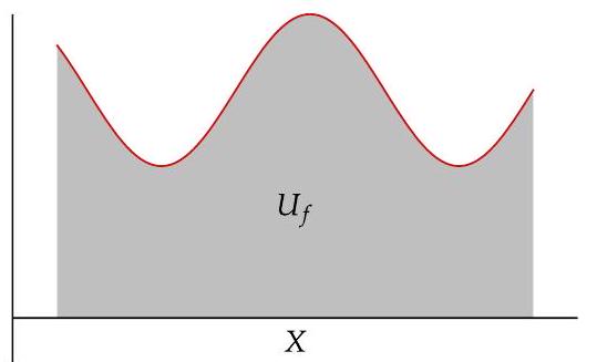
The figure indicates why we call U_{f} the region under the graph of f, even in cases when X is not a subset of \mathbf{R}. Similarly, the informal term area in the next paragraph should remind you of the area in the figure, even though we are really dealing with the measure of U_{f} in a product space.

The first equality in the result below can be thought of as recovering Riemann's conception of the integral as the area under the graph (although now in a much more general context with arbitrary $\sigma$-finite measures). The second equality in the result below can be thought of as reinforcing Lebesgue's conception of computing the area under a curve by integrating in the direction perpendicular to Riemann's.

5.35 area under the graph of a function equals the integral

Suppose (X, \mathcal{S}, \mu) is a $\sigma$-finite measure space and f: X \rightarrow[0, \infty] is an $\mathcal{S}$-measurable function. Let \mathcal{B} denote the $\sigma$-algebra of Borel subsets of (0, \infty), and let \lambda denote Lebesgue measure on ((0, \infty), \mathcal{B}). Then U_{f} \in \mathcal{S} \otimes \mathcal{B} and

(\mu \times \lambda)\left(U_{f}\right)=\int_{X} f d \mu=\int_{(0, \infty)} \mu({x \in X: t<f(x)}) d \lambda(t)

Proof For k \in \mathbf{Z}^{+}, let

E_{k}=\bigcup_{m=0}^{k^{2}-1}\left(f^{-1}\left(\left[\frac{m}{k}, \frac{m+1}{k}\right)\right) \times\left(0, \frac{m}{k}\right)\right) \quad \text { and } \quad F_{k}=f^{-1}([k, \infty]) \times(0, k) \text {. }

Then E_{k} is a finite union of $\mathcal{S} \otimes \mathcal{B}$-measurable rectangles and F_{k} is an \mathcal{S} \otimes \mathcal{B} measurable rectangle. Because

U_{f}=\bigcup_{k=1}^{\infty}\left(E_{k} \cup F_{k}\right)

we conclude that U_{f} \in \mathcal{S} \otimes \mathcal{B}.

Now the definition of the product measure \mu \times \lambda implies that

\begin{aligned} (\mu \times \lambda)\left(U_{f}\right) & =\int_{X} \int_{(0, \infty)} \chi_{U_{f}}(x, t) d \lambda(t) d \mu(x) \ & =\int_{X} f(x) d \mu(x), \end{aligned}

which completes the proof of the first equality in the conclusion of this theorem.

Tonelli's Theorem (5.28) tells us that we can interchange the order of integration in the double integral above, getting

\begin{aligned} (\mu \times \lambda)\left(U_{f}\right) & =\int_{(0, \infty)} \int_{X} \chi_{U_{f}}(x, t) d \mu(x) d \lambda(t) \ & =\int_{(0, \infty)} \mu({x \in X: t<f(x)}) d \lambda(t) \end{aligned}

which completes the proof of the second equality in the conclusion of this theorem.

Markov's inequality (4.1) implies that if f and \mu are as in the result above, then

\mu({x \in X: f(x)>t}) \leq \frac{\int_{X} f d \mu}{t}

for all t>0. Thus if \int_{X} f d \mu<\infty, then the result above should be considered to be somewhat stronger than Markov's inequality (because \int_{(0, \infty)} \frac{1}{t} d \lambda(t)=\infty ).

EXERCISES 5B

1 (a) Let \lambda denote Lebesgue measure on [0,1]. Show that

\int_{[0,1]} \int_{[0,1]} \frac{x^{2}-y^{2}}{\left(x^{2}+y^{2}\right)^{2}} d \lambda(y) d \lambda(x)=\frac{\pi}{4}

and

\int_{[0,1]} \int_{[0,1]} \frac{x^{2}-y^{2}}{\left(x^{2}+y^{2}\right)^{2}} d \lambda(x) d \lambda(y)=-\frac{\pi}{4}

(b) Explain why (a) violates neither Tonelli's Theorem nor Fubini's Theorem.

2 (a) Give an example of a doubly indexed collection $\left{x_{m, n}: m, n \in \mathbf{Z}^{+}\right}$of real numbers such that

\sum_{m=1}^{\infty} \sum_{n=1}^{\infty} x_{m, n}=0 \quad \text { and } \quad \sum_{n=1}^{\infty} \sum_{m=1}^{\infty} x_{m, n}=\infty

(b) Explain why (a) violates neither Tonelli's Theorem nor Fubini's Theorem.

3 Suppose (X, \mathcal{S}) is a measurable space and f: X \rightarrow[0, \infty] is a function. Let \mathcal{B} denote the $\sigma$-algebra of Borel subsets of (0, \infty). Prove that U_{f} \in \mathcal{S} \otimes \mathcal{B} if and only if f is an $\mathcal{S}$-measurable function.

4 Suppose (X, \mathcal{S}) is a measurable space and f: X \rightarrow \mathbf{R} is a function. Let \operatorname{graph}(f) \subset X \times \mathbf{R} denote the graph of f:

\operatorname{graph}(f)={(x, f(x)): x \in X} \text {. }

Let \mathcal{B} denote the $\sigma$-algebra of Borel subsets of \mathbf{R}. Prove that graph (f) \in \mathcal{S} \otimes \mathcal{B} if f is an $\mathcal{S}$-measurable function.

5 C Lebesgue Integration on \mathbf{R}^{n}

Throughout this section, assume that m and n are positive integers. Thus, for example, 5.36 should include the hypothesis that m and n are positive integers, but theorems and definitions become easier to state without explicitly repeating this hypothesis.

Borel Subsets of \mathbf{R}^{n}

We begin with a quick review of notation and key concepts concerning \mathbf{R}^{n}.

Recall that \mathbf{R}^{n} is the set of all $n$-tuples of real numbers:

\mathbf{R}^{n}=\left{\left(x_{1}, \ldots, x_{n}\right): x_{1}, \ldots, x_{n} \in \mathbf{R}\right}

The function \|\cdot\|_{\infty} from \mathbf{R}^{n} to [0, \infty) is defined by

\left|\left(x_{1}, \ldots, x_{n}\right)\right|{\infty}=\max \left{\left|x{1}\right|, \ldots,\left|x_{n}\right|\right}

For x \in \mathbf{R}^{n} and \delta>0, the open cube B(x, \delta) with side length 2 \delta is defined by

B(x, \delta)=\left{y \in \mathbf{R}^{n}:|y-x|_{\infty}<\delta\right} .

If n=1, then an open cube is simply a bounded open interval. If n=2, then an open cube might more appropriately be called an open square. However, using the cube terminology for all dimensions has the advantage of not requiring a different word for different dimensions.

A subset G of \mathbf{R}^{n} is called open if for every x \in G, there exists \delta>0 such that B(x, \delta) \subset G. Equivalently, a subset G of \mathbf{R}^{n} is called open if every element of G is contained in an open cube that is contained in G.

The union of every collection (finite or infinite) of open subsets of \mathbf{R}^{n} is an open subset of \mathbf{R}^{n}. Also, the intersection of every finite collection of open subsets of \mathbf{R}^{n} is an open subset of \mathbf{R}^{n}.

A subset of \mathbf{R}^{n} is called closed if its complement in \mathbf{R}^{n} is open. A set A \subset \mathbf{R}^{n} is called bounded if \sup \left\{\|a\|_{\infty}: a \in A\right\}<\infty.

We adopt the following common convention:

\mathbf{R}^{m} \times \mathbf{R}^{n} \text { is identified with } \mathbf{R}^{m+n} \text {. }

To understand the necessity of this convention, note that \mathbf{R}^{2} \times \mathbf{R} \neq \mathbf{R}^{3} because \mathbf{R}^{2} \times \mathbf{R} and \mathbf{R}^{3} contain different kinds of objects. Specifically, an element of \mathbf{R}^{2} \times \mathbf{R} is an ordered pair, the first of which is an element of \mathbf{R}^{2} and the second of which is an element of \mathbf{R}; thus an element of \mathbf{R}^{2} \times \mathbf{R} looks like \left(\left(x_{1}, x_{2}\right), x_{3}\right). An element of \mathbf{R}^{3} is an ordered triple of real numbers that looks like \left(x_{1}, x_{2}, x_{3}\right). However, we can identify \left(\left(x_{1}, x_{2}\right), x_{3}\right) with \left(x_{1}, x_{2}, x_{3}\right) in the obvious way. Thus we say that \mathbf{R}^{2} \times \mathbf{R} "equals" \mathbf{R}^{3}. More generally, we make the natural identification of \mathbf{R}^{m} \times \mathbf{R}^{n} with \mathbf{R}^{m+n}.

To check that you understand the identification discussed above, make sure that you see why B(x, \delta) \times B(y, \delta)=B((x, y), \delta) for all x \in \mathbf{R}^{m}, y \in \mathbf{R}^{n}, and \delta>0.

We can now prove that the product of two open sets is an open set.

5.36 product of open sets is open

Suppose G_{1} is an open subset of \mathbf{R}^{m} and G_{2} is an open subset of \mathbf{R}^{n}. Then G_{1} \times G_{2} is an open subset of \mathbf{R}^{m+n}.

Proof Suppose (x, y) \in G_{1} \times G_{2}. Then there exists an open cube D in \mathbf{R}^{m} centered at x and an open cube E in \mathbf{R}^{n} centered at y such that D \subset G_{1} and E \subset G_{2}. By reducing the size of either D or E, we can assume that the cubes D and E have the same side length. Thus D \times E is an open cube in \mathbf{R}^{m+n} centered at (x, y) that is contained in G_{1} \times G_{2}.

We have shown that an arbitrary point in G_{1} \times G_{2} is the center of an open cube contained in G_{1} \times G_{2}. Hence G_{1} \times G_{2} is an open subset of \mathbf{R}^{m+n}.

When n=1, the definition below of a Borel subset of \mathbf{R}^{1} agrees with our previous definition (2.29) of a Borel subset of \mathbf{R}.

5.37 Definition Borel set; \mathcal{B}_{n}

• A Borel subset of \mathbf{R}^{n} is an element of the smallest $\sigma$-algebra on \mathbf{R}^{n} containing all open subsets of \mathbf{R}^{n}.
• The $\sigma$-algebra of Borel subsets of \mathbf{R}^{n} is denoted by \mathcal{B}_{n}.

Recall that a subset of \mathbf{R} is open if and only if it is a countable disjoint union of open intervals. Part (a) in the result below provides a similar result in \mathbf{R}^{n}, although we must give up the disjoint aspect.

5.38 open sets are countable unions of open cubes

(a) A subset of \mathbf{R}^{n} is open in \mathbf{R}^{n} if and only if it is a countable union of open cubes in \mathbf{R}^{n}.

(b) \mathcal{B}_{n} is the smallest $\sigma$-algebra on \mathbf{R}^{n} containing all the open cubes in \mathbf{R}^{n}.

Proof We will prove (a), which clearly implies (b).

The proof that a countable union of open cubes is open is left as an exercise for the reader (actually, arbitrary unions of open cubes are open).

To prove the other direction, suppose G is an open subset of \mathbf{R}^{n}. For each x \in G, there is an open cube centered at x that is contained in G. Thus there is a smaller cube C_{x} such that x \in C_{x} \subset G and all coordinates of the center of C_{x} are rational numbers and the side length of C_{x} is a rational number. Now

G=\bigcup_{x \in G} C_{x} .

However, there are only countably many distinct cubes whose center has all rational coordinates and whose side length is rational. Thus G is the countable union of open cubes.

The next result tells us that the collection of Borel sets from various dimensions fit together nicely.

5.39 product of the Borel subsets of \mathbf{R}^{m} and the Borel subsets of \mathbf{R}^{n}

\mathcal{B}_{m} \otimes \mathcal{B}_{n}=\mathcal{B}_{m+n}

Proof Suppose E is an open cube in \mathbf{R}^{m+n}. Thus E is the product of an open cube in \mathbf{R}^{m} and an open cube in \mathbf{R}^{n}. Hence E \in \mathcal{B}_{m} \otimes \mathcal{B}_{n}. Thus the smallest $\sigma$-algebra containing all the open cubes in \mathbf{R}^{m+n} is contained in \mathcal{B}_{m} \otimes \mathcal{B}_{n}. Now 5.38(b) implies that \mathcal{B}_{m+n} \subset \mathcal{B}_{m} \otimes \mathcal{B}_{n}.

To prove the set inclusion in the other direction, temporarily fix an open set G in \mathbf{R}^{n}. Let

\mathcal{E}=\left{A \subset \mathbf{R}^{m}: A \times G \in \mathcal{B}_{m+n}\right} .

Then \mathcal{E} contains every open subset of \mathbf{R}^{m} (as follows from 5.36). Also, \mathcal{E} is closed under countable unions because

\left(\bigcup_{k=1}^{\infty} A_{k}\right) \times G=\bigcup_{k=1}^{\infty}\left(A_{k} \times G\right)

Furthermore, \mathcal{E} is closed under complementation because

\left(\mathbf{R}^{m} \backslash A\right) \times G=\left(\left(\mathbf{R}^{m} \times \mathbf{R}^{n}\right) \backslash(A \times G)\right) \cap\left(\mathbf{R}^{m} \times G\right)

Thus \mathcal{E} is a $\sigma$-algebra on \mathbf{R}^{m} that contains all open subsets of \mathbf{R}^{m}, which implies that \mathcal{B}_{m} \subset \mathcal{E}. In other words, we have proved that if A \in \mathcal{B}_{m} and G is an open subset of \mathbf{R}^{n}, then A \times G \in \mathcal{B}_{m+n}.

Now temporarily fix a Borel subset A of \mathbf{R}^{m}. Let

\mathcal{F}=\left{B \subset \mathbf{R}^{n}: A \times B \in \mathcal{B}_{m+n}\right}

The conclusion of the previous paragraph shows that \mathcal{F} contains every open subset of \mathbf{R}^{n}. As in the previous paragraph, we also see that \mathcal{F} is a $\sigma$-algebra. Hence \mathcal{B}_{n} \subset \mathcal{F}. In other words, we have proved that if A \in \mathcal{B}_{m} and B \in \mathcal{B}_{n}, then A \times B \in \mathcal{B}_{m+n}. Thus \mathcal{B}_{m} \otimes \mathcal{B}_{n} \subset \mathcal{B}_{m+n}, completing the proof.

The previous result implies a nice associative property. Specifically, if m, n, and p are positive integers, then two applications of 5.39 give

\left(\mathcal{B}{m} \otimes \mathcal{B}{n}\right) \otimes \mathcal{B}{p}=\mathcal{B}{m+n} \otimes \mathcal{B}{p}=\mathcal{B}{m+n+p}

Similarly, two more applications of 5.39 give

\mathcal{B}{m} \otimes\left(\mathcal{B}{n} \otimes \mathcal{B}{p}\right)=\mathcal{B}{m} \otimes \mathcal{B}{n+p}=\mathcal{B}{m+n+p}

Thus \left(\mathcal{B}_{m} \otimes \mathcal{B}_{n}\right) \otimes \mathcal{B}_{p}=\mathcal{B}_{m} \otimes\left(\mathcal{B}_{n} \otimes \mathcal{B}_{p}\right); hence we can dispense with parentheses when taking products of more than two Borel $\sigma$-algebras. More generally, we could have defined \mathcal{B}_{m} \otimes \mathcal{B}_{n} \otimes \mathcal{B}_{p} directly as the smallest $\sigma$-algebra on \mathbf{R}^{m+n+p} containing \left\{A \times B \times C: A \in \mathcal{B}_{m}, B \in \mathcal{B}_{n}, C \in \mathcal{B}_{p}\right\} and obtained the same $\sigma$-algebra (see Exercise 3 in this section).

Lebesgue Measure on \mathbf{R}^{n}

5.40 Definition Lebesgue measure; \lambda_{n}

Lebesgue measure on \mathbf{R}^{n} is denoted by \lambda_{n} and is defined inductively by

\lambda_{n}=\lambda_{n-1} \times \lambda_{1},

where \lambda_{1} is Lebesgue measure on \left(\mathbf{R}, \mathcal{B}_{1}\right).

Because \mathcal{B}_{n}=\mathcal{B}_{n-1} \otimes \mathcal{B}_{1} (by 5.39), the measure \lambda_{n} is defined on the Borel subsets of \mathbf{R}^{n}. Thinking of a typical point in \mathbf{R}^{n} as (x, y), where x \in \mathbf{R}^{n-1} and y \in \mathbf{R}, we can use the definition of the product of two measures (5.25) to write

\lambda_{n}(E)=\int_{\mathbf{R}^{n-1}} \int_{\mathbf{R}} \chi_{E}(x, y) d \lambda_{1}(y) d \lambda_{n-1}(x)

for E \in \mathcal{B}_{n}. Of course, we could use Tonelli's Theorem (5.28) to interchange the order of integration in the equation above.

Because Lebesgue measure is the most commonly used measure, mathematicians often dispense with explicitly displaying the measure and just use a variable name. In other words, if no measure is explicitly displayed in an integral and the context indicates no other measure, then you should assume that the measure involved is Lebesgue measure in the appropriate dimension. For example, the result of interchanging the order of integration in the equation above could be written as

\lambda_{n}(E)=\int_{\mathbf{R}} \int_{\mathbf{R}^{n-1}} \chi_{E}(x, y) d x d y

for E \in \mathcal{B}_{n}; here d x means d \lambda_{n-1}(x) and d y means d \lambda_{1}(y).

In the equations above giving formulas for \lambda_{n}(E), the integral over \mathbf{R}^{n-1} could be rewritten as an iterated integral over \mathbf{R}^{n-2} and \mathbf{R}, and that process could be repeated until reaching iterated integrals only over \mathbf{R}. Tonelli's Theorem could then be used repeatedly to swap the order of pairs of those integrated integrals, leading to iterated integrals in any order.

Similar comments apply to integrating functions on \mathbf{R}^{n} other than characteristic functions. For example, if f: \mathbf{R}^{3} \rightarrow \mathbf{R} is a $\mathcal{B}_{3}$-measurable function such that either f \geq 0 or \int_{\mathbf{R}^{3}}|f| d \lambda_{3}<\infty, then by either Tonelli's Theorem or Fubini's Theorem we have

\int_{\mathbf{R}^{3}} f d \lambda_{3}=\int_{\mathbf{R}} \int_{\mathbf{R}} \int_{\mathbf{R}} f\left(x_{1}, x_{2}, x_{3}\right) d x_{j} d x_{k} d x_{m},

where j, k, m is any permutation of 1,2,3.

Although we defined \lambda_{n} to be \lambda_{n-1} \times \lambda_{1}, we could have defined \lambda_{n} to be \lambda_{j} \times \lambda_{k} for any positive integers j, k with j+k=n. This potentially different definition would have led to the same $\sigma$-algebra \mathcal{B}_{n} (by 5.39) and to the same measure \lambda_{n} [because both potential definitions of \lambda_{n}(E) can be written as identical iterations of n integrals with respect to \lambda_{1} ].

Volume of Unit Ball in \mathbf{R}^{n}

The proof of the next result provides good experience in working with the Lebesgue measure \lambda_{n}. Recall that t E=\{t x: x \in E\}.

5.41 measure of a dilation

Suppose t>0. If E \in \mathcal{B}_{n}, then t E \in \mathcal{B}_{n} and \lambda_{n}(t E)=t^{n} \lambda_{n}(E).

Proof Let

\mathcal{E}=\left{E \in \mathcal{B}{n}: t E \in \mathcal{B}{n}\right}

Then \mathcal{E} contains every open subset of \mathbf{R}^{n} (because if E is open in \mathbf{R}^{n} then t E is open in \mathbf{R}^{n} ). Also, \mathcal{E} is closed under complementation and countable unions because

t\left(\mathbf{R}^{n} \backslash E\right)=\mathbf{R}^{n} \backslash(t E) \text { and } t\left(\bigcup_{k=1}^{\infty} E_{k}\right)=\bigcup_{k=1}^{\infty}\left(t E_{k}\right)

Hence \mathcal{E} is a $\sigma$-algebra on \mathbf{R}^{n} containing the open subsets of \mathbf{R}^{n}. Thus \mathcal{E}=\mathcal{B}_{n}. In other words, t E \in \mathcal{B}_{n} for all E \in \mathcal{B}_{n}.

To prove \lambda_{n}(t E)=t^{n} \lambda_{n}(E), first consider the case n=1. Lebesgue measure on \mathbf{R} is a restriction of outer measure. The outer measure of a set is determined by the sum of the lengths of countable collections of intervals whose union contains the set. Multiplying the set by t corresponds to multiplying each such interval by t, which multiplies the length of each such interval by t. In other words, \lambda_{1}(t E)=t \lambda_{1}(E).

Now assume n>1. We will use induction on n and assume that the desired result holds for n-1. If A \in \mathcal{B}_{n-1} and B \in \mathcal{B}_{1}, then

5.42

\begin{aligned} \lambda_{n}(t(A \times B)) & =\lambda_{n}((t A) \times(t B)) \ & =\lambda_{n-1}(t A) \cdot \lambda_{1}(t B) \ & =t^{n-1} \lambda_{n-1}(A) \cdot t \lambda_{1}(B) \ & =t^{n} \lambda_{n}(A \times B), \end{aligned}

giving the desired result for A \times B.

For m \in \mathbf{Z}^{+}, let C_{m} be the open cube in \mathbf{R}^{n} centered at the origin and with side length m. Let

\mathcal{E}{m}=\left{E \in \mathcal{B}{n}: E \subset C_{m} \text { and } \lambda_{n}(t E)=t^{n} \lambda_{n}(E)\right} \text {. }

From 5.42 and using 5.13(b), we see that finite unions of measurable rectangles contained in C_{m} are in \mathcal{E}_{m}. You should verify that \mathcal{E}_{m} is closed under countable increasing unions (use 2.59) and countable decreasing intersections (use 2.60, whose finite measure condition holds because we are working inside C_{m} ). From 5.13 and the Monotone Class Theorem (5.17), we conclude that \mathcal{E}_{m} is the $\sigma$-algebra on C_{m} consisting of Borel subsets of C_{m}. Thus \lambda_{n}(t E)=t^{n} \lambda_{n}(E) for all E \in \mathcal{B}_{n} such that E \subset C_{m}.

Now suppose E \in \mathcal{B}_{n}. Then 2.59 implies that

\lambda_{n}(t E)=\lim {m \rightarrow \infty} \lambda{n}\left(t\left(E \cap C_{m}\right)\right)=t^{n} \lim {m \rightarrow \infty} \lambda{n}\left(E \cap C_{m}\right)=t^{n} \lambda_{n}(E)

as desired.

5.43 Definition open unit ball in \mathbf{R}^{n} ; \mathbf{B}_{n}

The open unit ball in \mathbf{R}^{n} is denoted by \mathbf{B}_{n} and is defined by

\mathbf{B}{n}=\left{\left(x{1}, \ldots, x_{n}\right) \in \mathbf{R}^{n}: x_{1}{ }^{2}+\cdots+x_{n}{ }^{2}<1\right} .

The open unit ball \mathbf{B}_{n} is open in \mathbf{R}^{n} (as you should verify) and thus is in the collection \mathcal{B}_{n} of Borel sets.

5.44 volume of the unit ball in \mathbf{R}^{n}

\lambda_{n}\left(\mathbf{B}_{n}\right)= \begin{cases}\frac{\pi^{n / 2}}{(n / 2) !} & \text { if } n \text { is even, } \ \frac{2^{(n+1) / 2} \pi^{(n-1) / 2}}{1 \cdot 3 \cdot 5 \cdots \cdot n} & \text { if } n \text { is odd. }\end{cases}

Proof Because \lambda_{1}\left(\mathbf{B}_{1}\right)=2 and \lambda_{2}\left(\mathbf{B}_{2}\right)=\pi, the claimed formula is correct when n=1 and when n=2.

Now assume that n>2. We will use induction on n, assuming that the claimed formula is true for smaller values of n. Think of \mathbf{R}^{n}=\mathbf{R}^{2} \times \mathbf{R}^{n-2} and \lambda_{n}=\lambda_{2} \times \lambda_{n-2}. Then

\lambda_{n}\left(\mathbf{B}{n}\right)=\int{\mathbf{R}^{2}} \int_{\mathbf{R}^{n-2}} \chi_{\mathbf{B}_{n}}(x, y) d y d x

Temporarily fix x=\left(x_{1}, x_{2}\right) \in \mathbf{R}^{2}. If x_{1}{ }^{2}+x_{2}{ }^{2} \geq 1, then \chi_{\mathbf{B}_{n}}(x, y)=0 for all y \in \mathbf{R}^{n-2}. If x_{1}{ }^{2}+x_{2}{ }^{2}<1 and y \in \mathbf{R}^{n-2}, then \chi_{\mathbf{B}_{n}}(x, y)=1 if and only if y \in\left(1-x_{1}{ }^{2}-x_{2}{ }^{2}\right)^{1 / 2} \mathbf{B}_{n-2}. Thus the inner integral in 5.45 equals

\lambda_{n-2}\left(\left(1-x_{1}^{2}-x_{2}^{2}\right)^{1 / 2} \mathbf{B}{n-2}\right) \chi{\mathbf{B}_{2}}(x),

which by 5.41 equals

\left(1-x_{1}^{2}-x_{2}^{2}\right)^{(n-2) / 2} \lambda_{n-2}\left(\mathbf{B}{n-2}\right) \chi{\mathbf{B}_{2}}(x) .

Thus 5.45 becomes the equation

\lambda_{n}\left(\mathbf{B}{n}\right)=\lambda{n-2}\left(\mathbf{B}{n-2}\right) \int{\mathbf{B}{2}}\left(1-x{1}^{2}-x_{2}^{2}\right)^{(n-2) / 2} d \lambda_{2}\left(x_{1}, x_{2}\right)

To evaluate this integral, switch to the usual polar coordinates that you learned about in calculus \left(d \lambda_{2}=r d r d \theta\right), getting

\begin{aligned} \lambda_{n}\left(\mathbf{B}{n}\right) & =\lambda{n-2}\left(\mathbf{B}{n-2}\right) \int{-\pi}^{\pi} \int_{0}^{1}\left(1-r^{2}\right)^{(n-2) / 2} r d r d \theta \ & =\frac{2 \pi}{n} \lambda_{n-2}\left(\mathbf{B}_{n-2}\right) . \end{aligned}

The last equation and the induction hypothesis give the desired result.

This table gives the first five values of \lambda_{n}\left(\mathbf{B}_{n}\right), using 5.44. The last column of this table gives a decimal approximation to \lambda_{n}\left(\mathbf{B}_{n}\right), accurate to two digits after the decimal point. From this table, you might guess that \lambda_{n}\left(\mathbf{B}_{n}\right) is an increasing function of n, especially because the smallest cube containing the ball \mathbf{B}_{n} has n dimensional Lebesgue measure 2^{n}. However, Exercise 12 in this section shows that \lambda_{n}\left(\mathbf{B}_{n}\right) behaves much differently.

n	\lambda_{n}\left(\mathbf{B}_{n}\right)	\approx \lambda_{n}\left(\mathbf{B}_{n}\right)
1	2	2.00
2	\pi	3.14
3	4 \pi / 3	4.19
4	\pi^{2} / 2	4.93
5	8 \pi^{2} / 15	5.26

Equality of Mixed Partial Derivatives Via Fubini's Theorem

5.46 Definition partial derivatives; D_{1} f and D_{2} f

Suppose G is an open subset of \mathbf{R}^{2} and f: G \rightarrow \mathbf{R} is a function. For (x, y) \in G, the partial derivatives \left(D_{1} f\right)(x, y) and \left(D_{2} f\right)(x, y) are defined by

\left(D_{1} f\right)(x, y)=\lim _{t \rightarrow 0} \frac{f(x+t, y)-f(x, y)}{t}

and

\left(D_{2} f\right)(x, y)=\lim _{t \rightarrow 0} \frac{f(x, y+t)-f(x, y)}{t}

if these limits exist.

Using the notation for the cross section of a function (see 5.7), we could write the definitions of D_{1} and D_{2} in the following form:

\left(D_{1} f\right)(x, y)=\left([f]^{y}\right)^{\prime}(x) \quad \text { and } \quad\left(D_{2} f\right)(x, y)=\left([f]_{x}\right)^{\prime}(y)

5.47 Example partial derivatives of x^{y}

Let G=\left\{(x, y) \in \mathbf{R}^{2}: x>0\right\} and define f: G \rightarrow \mathbf{R} by f(x, y)=x^{y}. Then

\left(D_{1} f\right)(x, y)=y x^{y-1} \quad \text { and } \quad\left(D_{2} f\right)(x, y)=x^{y} \ln x

as you should verify. Taking partial derivatives of those partial derivatives, we have

\left(D_{2}\left(D_{1} f\right)\right)(x, y)=x^{y-1}+y x^{y-1} \ln x

and

\left(D_{1}\left(D_{2} f\right)\right)(x, y)=x^{y-1}+y x^{y-1} \ln x

as you should also verify. The last two equations show that D_{1}\left(D_{2} f\right)=D_{2}\left(D_{1} f\right) as functions on G.

In the example above, the two mixed partial derivatives turn out to equal each other, even though the intermediate results look quite different. The next result shows that the behavior in the example above is typical rather than a coincidence.

Some proofs of the result below do not use Fubini's Theorem. However, Fubini's Theorem leads to the clean proof below.

The integrals that appear in the proof below make sense because continuous real-valued functions on \mathbf{R}^{2} are measurable (because for a continuous function, the inverse image of each open set is open) and because continuous real-valued func-

Although the continuity hypotheses in the result below can be slightly weakened, they cannot be eliminated, as shown by Exercise 14 in this section. tions on closed bounded subsets of \mathbf{R}^{2} are bounded.

5.48 equality of mixed partial derivatives

Suppose G is an open subset of \mathbf{R}^{2} and f: G \rightarrow \mathbf{R} is a function such that D_{1} f, D_{2} f, D_{1}\left(D_{2} f\right), and D_{2}\left(D_{1} f\right) all exist and are continuous functions on G. Then

D_{1}\left(D_{2} f\right)=D_{2}\left(D_{1} f\right)

on G.

Proof Fix (a, b) \in G. For \delta>0, let S_{\delta}=[a, a+\delta] \times[b, b+\delta]. If S_{\delta} \subset G, then

\begin{aligned} \int_{S_{\delta}} D_{1}\left(D_{2} f\right) d \lambda_{2} & =\int_{b}^{b+\delta} \int_{a}^{a+\delta}\left(D_{1}\left(D_{2} f\right)\right)(x, y) d x d y \ & =\int_{b}^{b+\delta}\left[\left(D_{2} f\right)(a+\delta, y)-\left(D_{2} f\right)(a, y)\right] d y \ & =f(a+\delta, b+\delta)-f(a+\delta, b)-f(a, b+\delta)+f(a, b), \end{aligned}

where the first equality comes from Fubini's Theorem (5.32) and the second and third equalities come from the Fundamental Theorem of Calculus.

A similar calculation of \int_{S_{\delta}} D_{2}\left(D_{1} f\right) d \lambda_{2} yields the same result. Thus

\int_{S_{\delta}}\left[D_{1}\left(D_{2} f\right)-D_{2}\left(D_{1} f\right)\right] d \lambda_{2}=0

for all \delta such that \mathcal{S}_{\delta} \subset G. If \left(D_{1}\left(D_{2} f\right)\right)(a, b)>\left(D_{2}\left(D_{1} f\right)\right)(a, b), then by the continuity of D_{1}\left(D_{2} f\right) and D_{2}\left(D_{1} f\right), the integrand in the equation above is positive on S_{\delta} for \delta sufficiently small, which contradicts the integral above equaling 0 . Similarly, the inequality \left(D_{1}\left(D_{2} f\right)\right)(a, b)<\left(D_{2}\left(D_{1} f\right)\right)(a, b) also contradicts the equation above for small \delta. Thus we conclude that

\left(D_{1}\left(D_{2} f\right)\right)(a, b)=\left(D_{2}\left(D_{1} f\right)\right)(a, b),

as desired.

EXERCISES 5C

1 Show that a set G \subset \mathbf{R}^{n} is open in \mathbf{R}^{n} if and only if for each \left(b_{1}, \ldots, b_{n}\right) \in G, there exists r>0 such that

\left{\left(a_{1}, \ldots, a_{n}\right) \in \mathbf{R}^{n}: \sqrt{\left(a_{1}-b_{1}\right)^{2}+\cdots+\left(a_{n}-b_{n}\right)^{2}}<r\right} \subset G .

2 Show that there exists a set E \subset \mathbf{R}^{2} (thinking of \mathbf{R}^{2} as equal to \mathbf{R} \times \mathbf{R} ) such that the cross sections [E]_{a} and [E]^{a} are open subsets of \mathbf{R} for every a \in \mathbf{R}, but E \notin \mathcal{B}_{2}.

3 Suppose (X, \mathcal{S}),(Y, \mathcal{T}), and (Z, \mathcal{U}) are measurable spaces. We can define \mathcal{S} \otimes \mathcal{T} \otimes \mathcal{U} to be the smallest $\sigma$-algebra on X \times Y \times Z that contains

{A \times B \times C: A \in \mathcal{S}, B \in \mathcal{T}, C \in \mathcal{U}} .

Prove that if we make the obvious identifications of the products (X \times Y) \times Z and X \times(Y \times Z) with X \times Y \times Z, then

\mathcal{S} \otimes \mathcal{T} \otimes \mathcal{U}=(\mathcal{S} \otimes \mathcal{T}) \otimes \mathcal{U}=\mathcal{S} \otimes(\mathcal{T} \otimes \mathcal{U})

4 Show that Lebesgue measure on \mathbf{R}^{n} is translation invariant. More precisely, show that if E \in \mathcal{B}_{n} and a \in \mathbf{R}^{n}, then a+E \in \mathcal{B}_{n} and \lambda_{n}(a+E)=\lambda_{n}(E), where

a+E={a+x: x \in E} .

5 Suppose f: \mathbf{R}^{n} \rightarrow \mathbf{R} is $\mathcal{B}_{n}$-measurable and t \in \mathbf{R} \backslash\{0\}. Define f_{t}: \mathbf{R}^{n} \rightarrow \mathbf{R} by f_{t}(x)=f(t x).

(a) Prove that f_{t} is $\mathcal{B}_{n}$-measurable.

(b) Prove that if \int_{\mathbf{R}^{n}} f d \lambda_{n} is defined, then

\int_{\mathbf{R}^{n}} f_{t} d \lambda_{n}=\frac{1}{|t|^{n}} \int_{\mathbf{R}^{n}} f d \lambda_{n}

6 Suppose \lambda denotes Lebesgue measure on (\mathbf{R}, \mathcal{L}), where \mathcal{L} is the $\sigma$-algebra of Lebesgue measurable subsets of \mathbf{R}. Show that there exist subsets E and F of \mathbf{R}^{2} such that

• F \in \mathcal{L} \otimes \mathcal{L} and (\lambda \times \lambda)(F)=0;
• E \subset F but E \notin \mathcal{L} \otimes \mathcal{L}.

[The measure space (\mathbf{R}, \mathcal{L}, \lambda) has the property that every subset of a set with measure 0 is measurable. This exercise asks you to show that the measure space \left(\mathbf{R}^{2}, \mathcal{L} \otimes \mathcal{L}, \lambda \times \lambda\right) does not have this property. ]

7 Suppose m \in \mathbf{Z}^{+}. Verify that the collection of sets \mathcal{E}_{m} that appears in the proof of 5.41 is a monotone class.

8 Show that the open unit ball in \mathbf{R}^{n} is an open subset of \mathbf{R}^{n}.

9 Suppose G_{1} is a nonempty subset of \mathbf{R}^{m} and G_{2} is a nonempty subset of \mathbf{R}^{n}. Prove that G_{1} \times G_{2} is an open subset of \mathbf{R}^{m} \times \mathbf{R}^{n} if and only if G_{1} is an open subset of \mathbf{R}^{m} and G_{2} is an open subset of \mathbf{R}^{n}.

[One direction of this result was already proved (see 5.36); both directions are stated here to make the result look prettier and to be comparable to the next exercise, where neither direction has been proved.]

10 Suppose F_{1} is a nonempty subset of \mathbf{R}^{m} and F_{2} is a nonempty subset of \mathbf{R}^{n}. Prove that F_{1} \times F_{2} is a closed subset of \mathbf{R}^{m} \times \mathbf{R}^{n} if and only if F_{1} is a closed subset of \mathbf{R}^{m} and F_{2} is a closed subset of \mathbf{R}^{n}.

11 Suppose E is a subset of \mathbf{R}^{m} \times \mathbf{R}^{n} and

A=\left{x \in \mathbf{R}^{m}:(x, y) \in E \text { for some } y \in \mathbf{R}^{n}\right} .

(a) Prove that if E is an open subset of \mathbf{R}^{m} \times \mathbf{R}^{n}, then A is an open subset of \mathbf{R}^{m}.

(b) Prove or give a counterexample: If E is a closed subset of \mathbf{R}^{m} \times \mathbf{R}^{n}, then A is a closed subset of \mathbf{R}^{m}.

12 (a) Prove that \lim _{n \rightarrow \infty} \lambda_{n}\left(\mathbf{B}_{n}\right)=0.

(b) Find the value of n that maximizes \lambda_{n}\left(\mathbf{B}_{n}\right).

13 For readers familiar with the gamma function \Gamma : Prove that

\lambda_{n}\left(\mathbf{B}_{n}\right)=\frac{\pi^{n / 2}}{\Gamma\left(\frac{n}{2}+1\right)}

for every positive integer n.

14 Define f: \mathbf{R}^{2} \rightarrow \mathbf{R} by

f(x, y)= \begin{cases}\frac{x y\left(x^{2}-y^{2}\right)}{x^{2}+y^{2}} & \text { if }(x, y) \neq(0,0) \ 0 & \text { if }(x, y)=(0,0)\end{cases}

(a) Prove that D_{1}\left(D_{2} f\right) and D_{2}\left(D_{1} f\right) exist everywhere on \mathbf{R}^{2}.

(b) Show that \left(D_{1}\left(D_{2} f\right)\right)(0,0) \neq\left(D_{2}\left(D_{1} f\right)\right)(0,0).

(c) Explain why (b) does not violate 5.48.

Chapter 6

Banach Spaces

We begin this chapter with a quick review of the essentials of metric spaces. Then we extend our results on measurable functions and integration to complex-valued functions. After that, we rapidly review the framework of vector spaces, which allows us to consider natural collections of measurable functions that are closed under addition and scalar multiplication.

Normed vector spaces and Banach spaces, which are introduced in the third section of this chapter, play a hugely important role in modern analysis. Most interest focuses on linear maps on these vector spaces. Key results about linear maps that we develop in this chapter include the Hahn-Banach Theorem, the Open Mapping Theorem, the Closed Graph Theorem, and the Principle of Uniform Boundedness.

Market square in Lwów, a city that has been in several countries because of changing international boundaries. Before World War I, Lwów was in Austria-Hungary. During the period between World War I and World War II, Lwów was in Poland. During this time, mathematicians in Lwów, particularly Stefan Banach (1892-1945) and his colleagues, developed the basic results of modern functional analysis. After World War II, Lwów was in the USSR. Now Lwów is in Ukraine and is called Lviv.

CC-BY-SA Petar Milošević

6A Metric Spaces

Open Sets, Closed Sets, and Continuity

Much of analysis takes place in the context of a metric space, which is a set with a notion of distance that satisfies certain properties. The properties we would like a distance function to have are captured in the next definition, where you should think of d(f, g) as measuring the distance between f and g.

Specifically, we would like the distance between two elements of our metric space to be a nonnegative number that is 0 if and only if the two elements are the same. We would like the distance between two elements not to depend on the order in which we list them. Finally, we would like a triangle inequality (the last bullet point below), which states that the distance between two elements is less than or equal to the sum of the distances obtained when we insert an intermediate element.

Now we are ready for the formal definition.

6.1 Definition metric space

A metric on a nonempty set V is a function d: V \times V \rightarrow[0, \infty) such that

• d(f, f)=0 for all f \in V;
• if f, g \in V and d(f, g)=0, then f=g;
• d(f, g)=d(g, f) for all f, g \in V;
• d(f, h) \leq d(f, g)+d(g, h) for all f, g, h \in V.

A metric space is a pair (V, d), where V is a nonempty set and d is a metric on V.

6.2 Example metric spaces

• Suppose V is a nonempty set. Define d on V \times V by setting d(f, g) to be 1 if f \neq g and to be 0 if f=g. Then d is a metric on V.
• Define d on \mathbf{R} \times \mathbf{R} by d(x, y)=|x-y|. Then d is a metric on \mathbf{R}.
• For n \in \mathbf{Z}^{+}, define d on \mathbf{R}^{n} \times \mathbf{R}^{n} by

d\left(\left(x_{1}, \ldots, x_{n}\right),\left(y_{1}, \ldots, y_{n}\right)\right)=\max \left{\left|x_{1}-y_{1}\right|, \ldots,\left|x_{n}-y_{n}\right|\right} .

Then d is a metric on \mathbf{R}^{n}.

• Define d on C([0,1]) \times C([0,1]) by d(f, g)=\sup \{|f(t)-g(t)|: t \in[0,1]\}; here C([0,1]) is the set of continuous real-valued functions on [0,1]. Then d is a metric on C([0,1]).
• Define d on \ell^{1} \times \ell^{1} by d\left(\left(a_{1}, a_{2}, \ldots\right),\left(b_{1}, b_{2}, \ldots\right)\right)=\sum_{k=1}^{\infty}\left|a_{k}-b_{k}\right|; here \ell^{1} is the set of sequences \left(a_{1}, a_{2}, \ldots\right) of real numbers such that \sum_{k=1}^{\infty}\left|a_{k}\right|<\infty. Then d is a metric on \ell.

The material in this section is probably review for most readers of this book. Thus more details than usual are left to the reader to verify. Verifying those details and doing the exercises is the best way to solidify your understanding of these concepts. You should be able to transfer familiar definitions and proofs from the

This book often uses symbols such as f, g, h as generic elements of a generic metric space because many of the important metric spaces in analysis are sets of functions; for example, see the fourth bullet point of Example 6.2. context of \mathbf{R} or \mathbf{R}^{n} to the context of a metric space.

We will need to use a metric space's topological features, which we introduce now.

6.3 Definition open ball; B(f, r); closed ball; \bar{B}(f, r)

Suppose (V, d) is a metric space, f \in V, and r>0.

• The open ball centered at f with radius r is denoted B(f, r) and is defined by

B(f, r)={g \in V: d(f, g)<r} .

• The closed ball centered at f with radius r is denoted \bar{B}(f, r) and is defined by

\bar{B}(f, r)={g \in V: d(f, g) \leq r} .

Abusing terminology, many books (including this one) include phrases such as suppose V is a metric space without mentioning the metric d. When that happens, you should assume that a metric d lurks nearby, even if it is not explicitly named.

Our next definition declares a subset of a metric space to be open if every element in the subset is the center of an open ball that is contained in the set.

6.4 Definition open

A subset G of a metric space V is called open if for every f \in G, there exists r>0 such that B(f, r) \subset G.

6.5 open balls are open

Suppose V is a metric space, f \in V, and r>0. Then B(f, r) is an open subset of V.

Proof Suppose g \in B(f, r). We need to show that an open ball centered at g is contained in B(f, r). To do this, note that if h \in B(g, r-d(f, g)), then

d(f, h) \leq d(f, g)+d(g, h)<d(f, g)+(r-d(f, g))=r,

which implies that h \in B(f, r). Thus B(g, r-d(f, g)) \subset B(f, r), which implies that B(f, r) is open.

Closed sets are defined in terms of open sets.

6.6 Definition closed

A subset of a metric space V is called closed if its complement in V is open.

For example, each closed ball \bar{B}(f, r) in a metric space is closed, as you are asked to prove in Exercise 3.

Now we define the closure of a subset of a metric space.

6.7 Definition closure; \bar{E}

Suppose V is a metric space and E \subset V. The closure of E, denoted \bar{E}, is defined by

\bar{E}={g \in V: B(g, \varepsilon) \cap E \neq \varnothing \text { for every } \varepsilon>0} .

Limits in a metric space are defined by reducing to the context of real numbers, where limits have already been defined.

6.8 Definition limit in metric space; \lim _{k \rightarrow \infty} f_{k}

Suppose (V, d) is a metric space, f_{1}, f_{2}, \ldots is a sequence in V, and f \in V. Then

\lim {k \rightarrow \infty} f{k}=f \text { means } \lim {k \rightarrow \infty} d\left(f{k}, f\right)=0 \text {. }

In other words, a sequence f_{1}, f_{2}, \ldots in V converges to f \in V if for every \varepsilon>0, there exists $n \in \mathbf{Z}^{+}$such that

d\left(f_{k}, f\right)<\varepsilon \text { for all integers } k \geq n \text {. }

The next result states that the closure of a set is the collection of all limits of elements of the set. Also, a set is closed if and only if it equals its closure. The proof of the next result is left as an exercise that provides good practice in using these concepts.

6.9 closure

Suppose V is a metric space and E \subset V. Then

(a) \bar{E}=\left\{g \in V\right. : there exist f_{1}, f_{2}, \ldots in E such that \left.\lim _{k \rightarrow \infty} f_{k}=g\right\};

(b) \bar{E} is the intersection of all closed subsets of V that contain E;

(c) \bar{E} is a closed subset of V;

(d) E is closed if and only if \bar{E}=E;

(e) E is closed if and only if E contains the limit of every convergent sequence of elements of E.

The definition of continuity that follows uses the same pattern as the definition for a function from a subset of \mathbf{R} to \mathbf{R}.

6.10 Definition continuous

Suppose \left(V, d_{V}\right) and \left(W, d_{W}\right) are metric spaces and T: V \rightarrow W is a function.

• For f \in V, the function T is called continuous at f if for every \varepsilon>0, there exists \delta>0 such that

d_{W}(T(f), T(g))<\varepsilon

for all g \in V with d_{V}(f, g)<\delta.

• The function T is called continuous if T is continuous at f for every f \in V.

The next result gives equivalent conditions for continuity. Recall that T^{-1}(E) is called the inverse image of E and is defined to be \{f \in V: T(f) \in E\}. Thus the equivalence of the (a) and (c) below could be restated as saying that a function is continuous if and only if the inverse image of every open set is open. The equivalence of the (a) and (d) below could be restated as saying that a function is continuous if and only if the inverse image of every closed set is closed.

6.11 equivalent conditions for continuity

Suppose V and W are metric spaces and T: V \rightarrow W is a function. Then the following are equivalent:

(a) T is continuous.

(b) \lim _{k \rightarrow \infty} f_{k}=f in V implies \lim _{k \rightarrow \infty} T\left(f_{k}\right)=T(f) in W.

(c) T^{-1}(G) is an open subset of V for every open set G \subset W.

(d) T^{-1}(F) is a closed subset of V for every closed set F \subset W.

Proof We first prove that (b) implies (d). Suppose (b) holds. Suppose F is a closed subset of W. We need to prove that T^{-1}(F) is closed. To do this, suppose f_{1}, f_{2}, \ldots is a sequence in T^{-1}(F) and \lim _{k \rightarrow \infty} f_{k}=f for some f \in V. Because (b) holds, we know that \lim _{k \rightarrow \infty} T\left(f_{k}\right)=T(f). Because f_{k} \in T^{-1}(F) for each k \in \mathbf{Z}^{+}, we know that T\left(f_{k}\right) \in F for each k \in \mathbf{Z}^{+}. Because F is closed, this implies that T(f) \in F. Thus f \in T^{-1}(F), which implies that T^{-1}(F) is closed [by 6.9(e)], completing the proof that (b) implies (d).

The proof that (c) and (d) are equivalent follows from the equation

T^{-1}(W \backslash E)=V \backslash T^{-1}(E)

for every E \subset W and the fact that a set is open if and only if its complement (in the appropriate metric space) is closed.

The proof of the remaining parts of this result are left as an exercise that should help strengthen your understanding of these concepts.

Cauchy Sequences and Completeness

The next definition is useful for showing (in some metric spaces) that a sequence has a limit, even when we do not have a good candidate for that limit.

6.12 Definition Cauchy sequence

A sequence f_{1}, f_{2}, \ldots in a metric space (V, d) is called a Cauchy sequence if for every \varepsilon>0, there exists $n \in \mathbf{Z}^{+}$such that d\left(f_{j}, f_{k}\right)<\varepsilon for all integers j \geq n and k \geq n.

6.13 every convergent sequence is a Cauchy sequence

Every convergent sequence in a metric space is a Cauchy sequence.

Proof Suppose \lim _{k \rightarrow \infty} f_{k}=f in a metric space (V, d). Suppose \varepsilon>0. Then there exists $n \in \mathbf{Z}^{+}$such that d\left(f_{k}, f\right)<\frac{\varepsilon}{2} for all k \geq n. If $j, k \in \mathbf{Z}^{+}$are such that j \geq n and k \geq n, then

d\left(f_{j}, f_{k}\right) \leq d\left(f_{j}, f\right)+d\left(f, f_{k}\right)<\frac{\varepsilon}{2}+\frac{\varepsilon}{2}=\varepsilon .

Thus f_{1}, f_{2}, \ldots is a Cauchy sequence, completing the proof.

Metric spaces that satisfy the converse of the result above have a special name.

6.14 Definition complete metric space

A metric space V is called complete if every Cauchy sequence in V converges to some element of V.

6.15 Example

• All five of the metric spaces in Example 6.2 are complete, as you should verify.
• The metric space \mathbf{Q}, with metric defined by d(x, y)=|x-y|, is not complete. To see this, for $k \in \mathbf{Z}^{+}$let

x_{k}=\frac{1}{10^{1 !}}+\frac{1}{10^{2 !}}+\cdots+\frac{1}{10^{k !}} \text {. }

If j<k, then

\left|x_{k}-x_{j}\right|=\frac{1}{10^{(j+1) !}}+\cdots+\frac{1}{10^{k !}}<\frac{2}{10^{(j+1) !}} .

Thus x_{1}, x_{2}, \ldots is a Cauchy sequence in \mathbf{Q}. However, x_{1}, x_{2}, \ldots does not converge to an element of \mathbf{Q} because the limit of this sequence would have a decimal expansion 0.110001000000000000000001 \ldots that is neither a terminating decimal nor a repeating decimal. Thus \mathbf{Q} is not a complete metric space.

Entrance to the École Polytechnique (Paris), where Augustin-Louis Cauchy (1789-1857) was a student and a faculty member. Cauchy wrote almost 800 mathematics papers and the highly influential textbook Cours d'Analyse (published in 1821), which greatly influenced the development of analysis.

CC-BY-SA NonOmnisMoriar

Every nonempty subset of a metric space is a metric space. Specifically, suppose (V, d) is a metric space and U is a nonempty subset of V. Then restricting d to U \times U gives a metric on U. Unless stated otherwise, you should assume that the metric on a subset is this restricted metric that the subset inherits from the bigger set.

Combining the two bullet points in the result below shows that a subset of a complete metric space is complete if and only if it is closed.

6.16 connection between complete and closed

(a) A complete subset of a metric space is closed.

(b) A closed subset of a complete metric space is complete.

Proof We begin with a proof of (a). Suppose U is a complete subset of a metric space V. Suppose f_{1}, f_{2}, \ldots is a sequence in U that converges to some g \in V. Then f_{1}, f_{2}, \ldots is a Cauchy sequence in U (by 6.13). Hence by the completeness of U, the sequence f_{1}, f_{2}, \ldots converges to some element of U, which must be g (see Exercise 7). Hence g \in U. Now 6.9(e) implies that U is a closed subset of V, completing the proof of (a).

To prove (b), suppose U is a closed subset of a complete metric space V. To show that U is complete, suppose f_{1}, f_{2}, \ldots is a Cauchy sequence in U. Then f_{1}, f_{2}, \ldots is also a Cauchy sequence in V. By the completeness of V, this sequence converges to some f \in V. Because U is closed, this implies that f \in U (see 6.9). Thus the Cauchy sequence f_{1}, f_{2}, \ldots converges to an element of U, showing that U is complete. Hence (b) has been proved.

EXERCISES 6 A

1 Verify that each of the claimed metrics in Example 6.2 is indeed a metric.

2 Prove that every finite subset of a metric space is closed.

3 Prove that every closed ball in a metric space is closed.

4 Suppose V is a metric space.

(a) Prove that the union of each collection of open subsets of V is an open subset of V.

(b) Prove that the intersection of each finite collection of open subsets of V is an open subset of V.

5 Suppose V is a metric space.

(a) Prove that the intersection of each collection of closed subsets of V is a closed subset of V.

(b) Prove that the union of each finite collection of closed subsets of V is a closed subset of V.

6 (a) Prove that if V is a metric space, f \in V, and r>0, then \overline{B(f, r)} \subset \bar{B}(f, r).

(b) Give an example of a metric space V, f \in V, and r>0 such that \overline{B(f, r)} \neq \bar{B}(f, r).

7 Show that each sequence in a metric space has at most one limit.

8 Prove 6.9.

9 Prove that each open subset of a metric space V is the union of some sequence of closed subsets of V.

10 Prove or give a counterexample: If V is a metric space and U, W are subsets of V, then \bar{U} \cup \bar{W}=\overline{U \cup W}.

11 Prove or give a counterexample: If V is a metric space and U, W are subsets of V, then \bar{U} \cap \bar{W}=\overline{U \cap W}.

12 Suppose \left(U, d_{U}\right),\left(V, d_{V}\right), and \left(W, d_{W}\right) are metric spaces. Suppose also that T: U \rightarrow V and S: V \rightarrow W are continuous functions.

(a) Using the definition of continuity, show that S \circ T: U \rightarrow W is continuous.

(b) Using the equivalence of 6.11(a) and 6.11(b), show that S \circ T: U \rightarrow W is continuous.

(c) Using the equivalence of 6.11(a) and 6.11(c), show that S \circ T: U \rightarrow W is continuous.

13 Prove the parts of 6.11 that were not proved in the text.

14 Suppose a Cauchy sequence in a metric space has a convergent subsequence. Prove that the Cauchy sequence converges.

15 Verify that all five of the metric spaces in Example 6.2 are complete metric spaces.

16 Suppose (U, d) is a metric space. Let W denote the set of all Cauchy sequences of elements of U.

(a) For \left(f_{1}, f_{2}, \ldots\right) and \left(g_{1}, g_{2}, \ldots\right) in W, define \left(f_{1}, f_{2}, \ldots\right) \equiv\left(g_{1}, g_{2}, \ldots\right) to mean that

\lim {k \rightarrow \infty} d\left(f{k}, g_{k}\right)=0

Show that \equiv is an equivalence relation on W.

(b) Let V denote the set of equivalence classes of elements of W under the equivalence relation above. For \left(f_{1}, f_{2}, \ldots\right) \in W, let \left(f_{1}, f_{2}, \ldots\right)^{\wedge} denote the equivalence class of \left(f_{1}, f_{2}, \ldots\right). Define d_{V}: V \times V \rightarrow[0, \infty) by

d_{V}\left(\left(f_{1}, f_{2}, \ldots\right)^{\wedge},\left(g_{1}, g_{2}, \ldots\right)^{\wedge}\right)=\lim {k \rightarrow \infty} d\left(f{k}, g_{k}\right) .

Show that this definition of d_{V} makes sense and that d_{V} is a metric on V.

(c) Show that \left(V, d_{V}\right) is a complete metric space.

(d) Show that the map from U to V that takes f \in U to (f, f, f, \ldots) preserves distances, meaning that

d(f, g)=d_{V}\left((f, f, f, \ldots)^{\wedge},(g, g, g, \ldots)^{\wedge}\right)

for all f, g \in U.

(e) Explain why (d) shows that every metric space is a subset of some complete metric space.

6B Vector Spaces

Integration of Complex-Valued Functions

Complex numbers were invented so that we can take square roots of negative numbers. The idea is to assume we have a square root of -1 , denoted i, that obeys the usual rules of arithmetic. Here are the formal definitions:

6.17 Definition complex numbers; C; addition and multiplication in C

• A complex number is an ordered pair (a, b), where a, b \in \mathbf{R}, but we write this as a+b i or a+i b.
• The set of all complex numbers is denoted by \mathbf{C} :

\mathbf{C}={a+b i: a, b \in \mathbf{R}} .

• Addition and multiplication in \mathbf{C} are defined by

\begin{gathered} (a+b i)+(c+d i)=(a+c)+(b+d) i \ (a+b i)(c+d i)=(a c-b d)+(a d+b c) i \end{gathered}

here a, b, c, d \in \mathbf{R}.

If a \in \mathbf{R}, then we identify a+0 i with a. Thus we think of \mathbf{R} as a subset of C. We also usually write 0+b i as b i, and we usually write 0+1 i as i. You should verify that i^{2}=-1.

With the definitions as above, \mathbf{C} satisfies the usual rules of arithmetic. Specifically, with addition and multiplication defined as above, \mathbf{C} is a field, as you should verify. Thus subtraction and division of complex numbers are defined as in any field.

The field \mathbf{C} cannot be made into an ordered field. However, the useful concept of an absolute value can still be defined

The symbol i was first used to denote \sqrt{-1} by Leonhard Euler (1707-1783) in 1777. on \mathbf{C}.

6.18 Definition real part; \operatorname{Re} z; imaginary part; \operatorname{Im} z ; absolute value; limits

Suppose z=a+b i, where a and b are real numbers.

• The real part of z, denoted \operatorname{Re} z, is defined by \operatorname{Re} z=a.
• The imaginary part of z, denoted \operatorname{Im} z, is defined by \operatorname{Im} z=b.
• The absolute value of z, denoted |z|, is defined by |z|=\sqrt{a^{2}+b^{2}}.
• If z_{1}, z_{2}, \ldots \in \mathbf{C} and L \in \mathbf{C}, then \lim _{k \rightarrow \infty} z_{k}=L means \lim _{k \rightarrow \infty}\left|z_{k}-L\right|=0.

For b a real number, the usual definition of |b| as a real number is consistent with the new definition just given of |b| with b thought of as a complex number. Note that if z_{1}, z_{2}, \ldots is a sequence of complex numbers and L \in \mathbf{C}, then

\lim {k \rightarrow \infty} z{k}=L \Longleftrightarrow \lim {k \rightarrow \infty} \operatorname{Re} z{k}=\operatorname{Re} L \text { and } \lim {k \rightarrow \infty} \operatorname{Im} z{k}=\operatorname{Im} L .

We will reduce questions concerning measurability and integration of a complexvalued function to the corresponding questions about the real and imaginary parts of the function. We begin this process with the following definition.

6.19 Definition measurable complex-valued function

Suppose (X, \mathcal{S}) is a measurable space. A function f: X \rightarrow \mathrm{C} is called $\mathcal{S}$-measurable if \operatorname{Re} f and \operatorname{Im} f are both $\mathcal{S}$-measurable functions.

See Exercise 5 in this section for two natural conditions that are equivalent to measurability for complex-valued functions.

We will make frequent use of the following result. See Exercise 6 in this section for algebraic combinations of complex-valued measurable functions.

6.20|f|^{p} is measurable if f is measurable

Suppose (X, \mathcal{S}) is a measurable space, f: X \rightarrow \mathbf{C} is an $\mathcal{S}$-measurable function, and 0<p<\infty. Then |f|^{p} is an $\mathcal{S}$-measurable function.

Proof The functions (\operatorname{Re} f)^{2} and (\operatorname{Im} f)^{2} are $\mathcal{S}$-measurable because the square of an $\mathcal{S}$-measurable function is measurable (by Example 2.45). Thus the function (\operatorname{Re} f)^{2}+(\operatorname{Im} f)^{2} is $\mathcal{S}$-measurable (because the sum of two $\mathcal{S}$-measurable functions is $\mathcal{S}$-measurable by 2.46). Now \left((\operatorname{Re} f)^{2}+(\operatorname{Im} f)^{2}\right)^{p / 2} is $\mathcal{S}$-measurable because it is the composition of a continuous function on [0, \infty) and an $\mathcal{S}$-measurable function (see 2.44 and 2.41). In other words, |f|^{p} is an $\mathcal{S}$-measurable function.

Now we define integration of a complex-valued function by separating the function into its real and imaginary parts.

6.21 Definition integral of a complex-valued function; \int f d \mu

Suppose (X, \mathcal{S}, \mu) is a measure space and f: X \rightarrow \mathbf{C} is an $\mathcal{S}$-measurable function with \int|f| d \mu<\infty [the collection of such functions is denoted \mathcal{L}^{1}(\mu) ]. Then \int f d \mu is defined by

\int f d \mu=\int(\operatorname{Re} f) d \mu+i \int(\operatorname{Im} f) d \mu .

The integral of a complex-valued measurable function is defined above only when the absolute value of the function has a finite integral. In contrast, the integral of every nonnegative measurable function is defined (although the value may be \infty ), and if f is real valued then \int f d \mu is defined to be \int f^{+} d \mu-\int f^{-} d \mu if at least one of \int f^{+} d \mu and \int f^{-} d \mu is finite.

You can easily show that if f, g: X \rightarrow \mathbf{C} are $\mathcal{S}$-measurable functions such that \int|f| d \mu<\infty and \int|g| d \mu<\infty, then

\int(f+g) d \mu=\int f d \mu+\int g d \mu .

Similarly, the definition of complex multiplication leads to the conclusion that

\int \alpha f d \mu=\alpha \int f d \mu

for all \alpha \in \mathbf{C} (see Exercise 8).

The inequality in the result below concerning integration of complex-valued functions does not follow immediately from the corresponding result for real-valued functions. However, the small trick used in the proof below does give a reasonably simple proof.

6.22 bound on the absolute value of an integral

Suppose (X, \mathcal{S}, \mu) is a measure space and f: X \rightarrow \mathbf{C} is an $\mathcal{S}$-measurable function such that \int|f| d \mu<\infty. Then

\left|\int f d \mu\right| \leq \int|f| d \mu

Proof The result clearly holds if \int f d \mu=0. Thus assume that \int f d \mu \neq 0.

Let

\alpha=\frac{\left|\int f d \mu\right|}{\int f d \mu}

Then

\begin{aligned} \left|\int f d \mu\right|=\alpha \int f d \mu & =\int \alpha f d \mu \ & =\int \operatorname{Re}(\alpha f) d \mu+i \int \operatorname{Im}(\alpha f) d \mu \ & =\int \operatorname{Re}(\alpha f) d \mu \ & \leq \int|\alpha f| d \mu \ & =\int|f| d \mu \end{aligned}

where the second equality holds by Exercise 8, the fourth equality holds because \left|\int f d \mu\right| \in \mathbf{R}, the inequality on the fourth line holds because \operatorname{Re} z \leq|z| for every complex number z, and the equality in the last line holds because |\alpha|=1.

Because of the result above, the Bounded Convergence Theorem (3.26) and the Dominated Convergence Theorem (3.31) hold if the functions f_{1}, f_{2}, \ldots and f in the statements of those theorems are allowed to be complex valued.

We now define the complex conjugate of a complex number.

6.23 Definition complex conjugate; \bar{z}

Suppose z \in \mathbf{C}. The complex conjugate of z \in \mathbf{C}, denoted \bar{z} (pronounced $z$-bar), is defined by

\bar{z}=\operatorname{Re} z-(\operatorname{Im} z) i

For example, if z=5+7 i then \bar{z}=5-7 i. Note that a complex number z is a real number if and only if z=\bar{z}.

The next result gives basic properties of the complex conjugate.

6.24 properties of complex conjugates

Suppose w, z \in \mathbf{C}. Then

• product of z and \bar{z}

z \bar{z}=|z|^{2}

• sum and difference of z and \bar{z}

z+\bar{z}=2 \operatorname{Re} z and z-\bar{z}=2(\operatorname{Im} z) i

• additivity and multiplicativity of complex conjugate

\overline{w+z}=\bar{w}+\bar{z} and \overline{w z}=\bar{w} \bar{z}

• complex conjugate of complex conjugate

\overline{\bar{z}}=z

• absolute value of complex conjugate

|\bar{z}|=|z|

• integral of complex conjugate of a function

\int \bar{f} d \mu=\overline{\int f d \mu} for every measure \mu and every f \in \mathcal{L}^{1}(\mu).

Proof The first item holds because

z \bar{z}=(\operatorname{Re} z+i \operatorname{Im} z)(\operatorname{Re} z-i \operatorname{Im} z)=(\operatorname{Re} z)^{2}+(\operatorname{Im} z)^{2}=|z|^{2}

To prove the last item, suppose \mu is a measure and f \in \mathcal{L}^{1}(\mu). Then

\begin{aligned} \int \bar{f} d \mu=\int(\operatorname{Re} f-i \operatorname{Im} f) d \mu & =\int \operatorname{Re} f d \mu-i \int \operatorname{Im} f d \mu \ & =\overline{\int \operatorname{Re} f d \mu+i \int \operatorname{Im} f d \mu} \ & =\overline{\int f d \mu}, \end{aligned}

as desired.

The straightforward proofs of the remaining items are left to the reader.

Vector Spaces and Subspaces

The structure and language of vector spaces will help us focus on certain features of collections of measurable functions. So that we can conveniently make definitions and prove theorems that apply to both real and complex numbers, we adopt the following notation.

6.25 Definition \mathbf{F}

From now on, \mathbf{F} stands for either \mathbf{R} or \mathbf{C}.

In the definitions that follow, we use f and g to denote elements of V because in the crucial examples the elements of V are functions from a set X to \mathbf{F}.

6.26 Definition addition; scalar multiplication

• An addition on a set V is a function that assigns an element f+g \in V to each pair of elements f, g \in V.
• A scalar multiplication on a set V is a function that assigns an element \alpha f \in V to each \alpha \in \mathbf{F} and each f \in V.

Now we are ready to give the formal definition of a vector space.

6.27 Definition vector space

A vector space (over \mathbf{F} ) is a set V along with an addition on V and a scalar multiplication on V such that the following properties hold:

commutativity

f+g=g+f for all f, g \in V;

associativity

(f+g)+h=f+(g+h) and (\alpha \beta) f=\alpha(\beta f) for all f, g, h \in V and \alpha, \beta \in \mathbf{F} ;

additive identity

there exists an element 0 \in V such that f+0=f for all f \in V;

additive inverse

for every f \in V, there exists g \in V such that f+g=0;

multiplicative identity

1 f=f for all f \in V

distributive properties

\alpha(f+g)=\alpha f+\alpha g and (\alpha+\beta) f=\alpha f+\beta f for all \alpha, \beta \in \mathbf{F} and f, g \in V.

Most vector spaces that you will encounter are subsets of the vector space \mathbf{F}^{X} presented in the next example.

6.28 Example the vector space \mathbf{F}^{X}

Suppose X is a nonempty set. Let \mathbf{F}^{X} denote the set of functions from X to \mathbf{F}. Addition and scalar multiplication on \mathbf{F}^{X} are defined as expected: for f, g \in \mathbf{F}^{X} and \alpha \in \mathbf{F}, define

(f+g)(x)=f(x)+g(x) \quad \text { and } \quad(\alpha f)(x)=\alpha(f(x))

for x \in X. Then, as you should verify, \mathbf{F}^{X} is a vector space; the additive identity in this vector space is the function 0 \in \mathbf{F}^{X} defined by 0(x)=0 for all x \in X.

6.29 Example \mathbf{F}^{n} ; \mathbf{F}^{\mathbf{Z}^{+}}

Special case of the previous example: if $n \in \mathbf{Z}^{+}$and X=\{1, \ldots, n\}, then \mathbf{F}^{X} is the familiar space \mathbf{R}^{n} or \mathbf{C}^{n}, depending upon whether \mathbf{F}=\mathbf{R} or \mathbf{F}=\mathbf{C}.

Another special case: \mathbf{F}^{\mathbf{Z}} is the vector space of all sequences of real numbers or complex numbers, again depending upon whether \mathbf{F}=\mathbf{R} or \mathbf{F}=\mathbf{C}.

By considering subspaces, we can greatly expand our examples of vector spaces.

6.30 Definition subspace

A subset U of V is called a subspace of V if U is also a vector space (using the same addition and scalar multiplication as on V ).

The next result gives the easiest way to check whether a subset of a vector space is a subspace.

6.31 conditions for a subspace

A subset U of V is a subspace of V if and only if U satisfies the following three conditions:

• additive identity 0 \in U

- closed under addition

f, g \in U implies f+g \in U;

• closed under scalar multiplication

\alpha \in \mathbf{F} and f \in U implies \alpha f \in U.

Proof If U is a subspace of V, then U satisfies the three conditions above by the definition of vector space.

Conversely, suppose U satisfies the three conditions above. The first condition above ensures that the additive identity of V is in U.

The second condition above ensures that addition makes sense on U. The third condition ensures that scalar multiplication makes sense on U.

If f \in V, then 0 f=(0+0) f=0 f+0 f. Adding the additive inverse of 0 f to both sides of this equation shows that 0 f=0. Now if f \in U, then (-1) f is also in U by the third condition above. Because f+(-1) f=(1+(-1)) f=0 f=0, we see that (-1) f is an additive inverse of f. Hence every element of U has an additive inverse in U.

The other parts of the definition of a vector space, such as associativity and commutativity, are automatically satisfied for U because they hold on the larger space V. Thus U is a vector space and hence is a subspace of V.

The three conditions in 6.31 usually enable us to determine quickly whether a given subset of V is a subspace of V, as illustrated below. All the examples below except for the first bullet point involve concepts from measure theory.

6.32 Example subspaces of \mathbf{F}^{X}

• The set C([0,1]) of continuous real-valued functions on [0,1] is a vector space over \mathbf{R} because the sum of two continuous functions is continuous and a constant multiple of a continuous functions is continuous. In other words, C([0,1]) is a subspace of \mathbf{R}^{[0,1]}.
• Suppose (X, \mathcal{S}) is a measurable space. Then the set of $\mathcal{S}$-measurable functions from X to \mathbf{F} is a subspace of \mathbf{F}^{X} because the sum of two $\mathcal{S}$-measurable functions is $\mathcal{S}$-measurable and a constant multiple of an $\mathcal{S}$-measurable function is \mathcal{S} measurable.
• Suppose (X, \mathcal{S}, \mu) is a measure space. Then the set \mathcal{Z}(\mu) of $\mathcal{S}$-measurable functions f from X to \mathbf{F} such that f=0 almost everywhere [meaning that \mu(\{x \in X: f(x) \neq 0\})=0] is a vector space over \mathbf{F} because the union of two sets with $\mu$-measure 0 is a set with $\mu$-measure 0 [which implies that \mathcal{Z}(\mu) is closed under addition]. Note that \mathcal{Z}(\mu) is a subspace of \mathbf{F}^{X}.
• Suppose (X, \mathcal{S}) is a measurable space. Then the set of bounded measurable functions from X to \mathbf{F} is a subspace of \mathbf{F}^{X} because the sum of two bounded $\mathcal{S}$-measurable functions is a bounded $\mathcal{S}$-measurable function and a constant multiple of a bounded $\mathcal{S}$-measurable function is a bounded $\mathcal{S}$-measurable function.
• Suppose (X, \mathcal{S}, \mu) is a measure space. Then the set of $\mathcal{S}$-measurable functions f from X to \mathbf{F} such that \int f d \mu=0 is a subspace of \mathbf{F}^{X} because of standard properties of integration.
• Suppose (X, \mathcal{S}, \mu) is a measure space. Then the set \mathcal{L}^{1}(\mu) of $\mathcal{S}$-measurable functions from X to \mathbf{F} such that \int|f| d \mu<\infty is a subspace of \mathbf{F}^{X} [we are now redefining \mathcal{L}^{1}(\mu) to allow for the possibility that \mathbf{F}=\mathbf{R} or \left.\mathbf{F}=\mathbf{C}\right]. The set \mathcal{L}^{1}(\mu) is closed under addition and scalar multiplication because \int|f+g| d \mu \leq \int|f| d \mu+\int|g| d \mu and \int|\alpha f| d \mu=|\alpha| \int|f| d \mu.
• The set \ell^{1} of all sequences \left(a_{1}, a_{2}, \ldots\right) of elements of \mathbf{F} such that \sum_{k=1}^{\infty}\left|a_{k}\right|<\infty is a subspace of \mathbf{F}^{\mathbf{Z}^{+}}. Note that \ell^{1} is a special case of the example in the previous bullet point (take \mu to be counting measure on \mathbf{Z}^{+}).

EXERCISES 6B

1 Show that if a, b \in \mathbf{R} with a+b i \neq 0, then

\frac{1}{a+b i}=\frac{a}{a^{2}+b^{2}}-\frac{b}{a^{2}+b^{2}} i

2 Suppose z \in C. Prove that

\max {|\operatorname{Re} z|,|\operatorname{Im} z|} \leq|z| \leq \sqrt{2} \max {|\operatorname{Re} z|,|\operatorname{Im} z|} .

3 Suppose z \in \mathbf{C}. Prove that \frac{|\operatorname{Re} z|+|\operatorname{Im} z|}{\sqrt{2}} \leq|z| \leq|\operatorname{Re} z|+|\operatorname{Im} z|.

4 Suppose w, z \in \mathbf{C}. Prove that |w z|=|w||z| and |w+z| \leq|w|+|z|.

5 Suppose (X, \mathcal{S}) is a measurable space and f: X \rightarrow \mathbf{C} is a complex-valued function. For conditions (b) and (c) below, identify \mathbf{C} with \mathbf{R}^{2}. Prove that the following are equivalent:

(a) f is $\mathcal{S}$-measurable.

(b) f^{-1}(G) \in \mathcal{S} for every open set G in \mathbf{R}^{2}.

(c) f^{-1}(B) \in \mathcal{S} for every Borel set B \in \mathcal{B}_{2}.

6 Suppose (X, \mathcal{S}) is a measurable space and f, g: X \rightarrow \mathbf{C} are $\mathcal{S}$-measurable. Prove that

(a) f+g, f-g, and f g are $\mathcal{S}$-measurable functions;

(b) if g(x) \neq 0 for all x \in X, then \frac{f}{g} is an $\mathcal{S}$-measurable function.

7 Suppose (X, \mathcal{S}) is a measurable space and f_{1}, f_{2}, \ldots is a sequence of \mathcal{S} measurable functions from X to C. Suppose \lim _{k \rightarrow \infty} f_{k}(x) exists for each x \in X. Define f: X \rightarrow \mathbf{C} by

f(x)=\lim {k \rightarrow \infty} f{k}(x)

Prove that f is an $\mathcal{S}$-measurable function.

8 Suppose (X, \mathcal{S}, \mu) is a measure space and f: X \rightarrow \mathbf{C} is an $\mathcal{S}$-measurable function such that \int|f| d \mu<\infty. Prove that if \alpha \in \mathbf{C}, then

\int \alpha f d \mu=\alpha \int f d \mu

9 Suppose V is a vector space. Show that the intersection of every collection of subspaces of V is a subspace of V.

10 Suppose V and W are vector spaces. Define V \times W by

V \times W={(f, g): f \in V \text { and } g \in W}

Define addition and scalar multiplication on V \times W by

\left(f_{1}, g_{1}\right)+\left(f_{2}, g_{2}\right)=\left(f_{1}+f_{2}, g_{1}+g_{2}\right) \quad \text { and } \quad \alpha(f, g)=(\alpha f, \alpha g) \text {. }

Prove that V \times W is a vector space with these operations.

6C Normed Vector Spaces

Norms and Complete Norms

This section begins with a crucial definition.

6.33 Definition norm; normed vector space

A norm on a vector space V( over \mathbf{F}) is a function \|\cdot\|: V \rightarrow[0, \infty) such that

• \|f\|=0 if and only if f=0 (positive definite);
• \|\alpha f\|=|\alpha|\|f\| for all \alpha \in \mathbf{F} and f \in V (homogeneity);
• \|f+g\| \leq\|f\|+\|g\| for all f, g \in V (triangle inequality).

A normed vector space is a pair (V,\|\cdot\|), where V is a vector space and \|\cdot\| is a norm on V.

6.34 Example norms

• Suppose n \in \mathbf{Z}^{+}. Define \|\cdot\|_{1} and \|\cdot\|_{\infty} on \mathbf{F}^{n} by

\left|\left(a_{1}, \ldots, a_{n}\right)\right|{1}=\left|a{1}\right|+\cdots+\left|a_{n}\right|

and

\left|\left(a_{1}, \ldots, a_{n}\right)\right|{\infty}=\max \left{\left|a{1}\right|, \ldots,\left|a_{n}\right|\right} .

Then \|\cdot\|_{1} and \|\cdot\|_{\infty} are norms on \mathbf{F}^{n}, as you should verify.

• On \ell^{1} (see the last bullet point in Example 6.32 for the definition of \ell^{1} ), define \|\cdot\|_{1} by

\left|\left(a_{1}, a_{2}, \ldots\right)\right|{1}=\sum{k=1}^{\infty}\left|a_{k}\right|

Then \|\cdot\|_{1} is a norm on \ell^{1}, as you should verify.

• Suppose X is a nonempty set and b(X) is the subspace of \mathbf{F}^{X} consisting of the bounded functions from X to \mathbf{F}. For f a bounded function from X to \mathbf{F}, define \|f\| by

|f|=\sup {|f(x)|: x \in X} .

Then \|\cdot\| is a norm on b(X), as you should verify.

• Let C([0,1]) denote the vector space of continuous functions from the interval [0,1] to \mathbf{F}. Define \|\cdot\| on C([0,1]) by

|f|=\int_{0}^{1}|f|

Then \|\cdot\| is a norm on C([0,1]), as you should verify.

Sometimes examples that do not satisfy a definition help you gain understanding.

6.35 Example not norms

• Let \mathcal{L}^{1}(\mathbf{R}) denote the vector space of Borel (or Lebesgue) measurable functions f: \mathbf{R} \rightarrow \mathbf{F} such that \int|f| d \lambda<\infty, where \lambda is Lebesgue measure on \mathbf{R}. Define \|\cdot\|_{1} on \mathcal{L}^{1}(\mathbf{R}) by

|f|_{1}=\int|f| d \lambda

Then \|\cdot\|_{1} satisfies the homogeneity condition and the triangle inequality on \mathcal{L}^{1}(\mathbf{R}), as you should verify. However, \|\cdot\|_{1} is not a norm on \mathcal{L}^{1}(\mathbf{R}) because the positive definite condition is not satisfied. Specifically, if E is a nonempty Borel subset of \mathbf{R} with Lebesgue measure 0 (for example, E might consist of a single element of \mathbf{R} ), then \left\|\chi_{E}\right\|_{1}=0 but \chi_{E} \neq 0. In the next chapter, we will discuss a modification of \mathcal{L}^{1}(\mathbf{R}) that removes this problem.

• If $n \in \mathbf{Z}^{+}$and \|\cdot\| is defined on \mathbf{F}^{n} by

\left|\left(a_{1}, \ldots, a_{n}\right)\right|=\left|a_{1}\right|^{1 / 2}+\cdots+\left|a_{n}\right|^{1 / 2},

then \|\cdot\| satisfies the positive definite condition and the triangle inequality (as you should verify). However, \|\cdot\| as defined above is not a norm because it does not satisfy the homogeneity condition.

• If \|\cdot\|_{1 / 2} is defined on \mathbf{F}^{n} by

\left|\left(a_{1}, \ldots, a_{n}\right)\right|{1 / 2}=\left(\left|a{1}\right|^{1 / 2}+\cdots+\left|a_{n}\right|^{1 / 2}\right)^{2},

then \|\cdot\|_{1 / 2} satisfies the positive definite condition and the homogeneity condition. However, if n>1 then \|\cdot\|_{1 / 2} is not a norm on \mathbf{F}^{n} because the triangle inequality is not satisfied (as you should verify).

The next result shows that every normed vector space is also a metric space in a natural fashion.

6.36 normed vector spaces are metric spaces

Suppose (V,\|\cdot\|) is a normed vector space. Define d: V \times V \rightarrow[0, \infty) by

d(f, g)=|f-g| \text {. }

Then d is a metric on V.

Proof Suppose f, g, h \in V. Then

\begin{aligned} d(f, h)=|f-h| & =|(f-g)+(g-h)| \ & \leq|f-g|+|g-h| \ & =d(f, g)+d(g, h) . \end{aligned}

Thus the triangle inequality requirement for a metric is satisfied. The verification of the other required properties for a metric are left to the reader.

From now on, all metric space notions in the context of a normed vector space should be interpreted with respect to the metric introduced in the previous result. However, usually there is no need to introduce the metric d explicitly—just use the norm of the difference of two elements. For example, suppose (V,\|\cdot\|) is a normed vector space, f_{1}, f_{2}, \ldots is a sequence in V, and f \in V. Then in the context of a normed vector space, the definition of limit (6.8) becomes the following statement:

\lim {k \rightarrow \infty} f{k}=f \text { means } \lim {k \rightarrow \infty}\left|f{k}-f\right|=0

As another example, in the context of a normed vector space, the definition of a Cauchy sequence (6.12) becomes the following statement:

A sequence f_{1}, f_{2}, \ldots in a normed vector space (V,\|\cdot\|) is a Cauchy sequence if for every \varepsilon>0, there exists $n \in \mathbf{Z}^{+}$such that \left\|f_{j}-f_{k}\right\|<\varepsilon for all integers j \geq n and k \geq n.

Every sequence in a normed vector space that has a limit is a Cauchy sequence (see 6.13). Normed vector spaces that satisfy the converse have a special name.

6.37 Definition Banach space

A complete normed vector space is called a Banach space.

In other words, a normed vector space V is a Banach space if every Cauchy sequence in V converges to some element of V.

The verifications of the assertions in Examples 6.38 and 6.39 below are left to the reader as exercises.

In a slight abuse of terminology, we often refer to a normed vector space V without mentioning the norm \|\cdot\|. When that happens, you should assume that a norm \|\cdot\| lurks nearby, even if it is not explicitly displayed.

6.38 Example Banach spaces

• The vector space C([0,1]) with the norm defined by \|f\|=\sup |f| is a Banach space.
• The vector space \ell^{1} with the norm defined by \left\|\left(a_{1}, a_{2}, \ldots\right)\right\|_{1}=\sum_{k=1}^{\infty}\left|a_{k}\right| is a Banach space.

6.39 Example not a Banach space

• The vector space C([0,1]) with the norm defined by \|f\|=\int_{0}^{1}|f| is not a Banach space.
• The vector space \ell^{1} with the norm defined by \left\|\left(a_{1}, a_{2}, \ldots\right)\right\|_{\infty}=\sup \left|a_{k}\right| is not a Banach space.

6.40 Definition infinite sum in a normed vector space

Suppose g_{1}, g_{2}, \ldots is a sequence in a normed vector space V. Then \sum_{k=1}^{\infty} g_{k} is defined by

\sum_{k=1}^{\infty} g_{k}=\lim {n \rightarrow \infty} \sum{k=1}^{n} g_{k}

if this limit exists, in which case the infinite series is said to converge.

Recall from your calculus course that if a_{1}, a_{2}, \ldots is a sequence of real numbers such that \sum_{k=1}^{\infty}\left|a_{k}\right|<\infty, then \sum_{k=1}^{\infty} a_{k} converges. The next result states that the analogous property for normed vector spaces characterizes Banach spaces.

6.41\left(\sum_{k=1}^{\infty}\left\|g_{k}\right\|<\infty \Longrightarrow \sum_{k=1}^{\infty} g_{k}\right. converges ) \Longleftrightarrow Banach space

Suppose V is a normed vector space. Then V is a Banach space if and only if \sum_{k=1}^{\infty} g_{k} converges for every sequence g_{1}, g_{2}, \ldots in V such that \sum_{k=1}^{\infty}\left\|g_{k}\right\|<\infty.

Proof First suppose V is a Banach space. Suppose g_{1}, g_{2}, \ldots is a sequence in V such that \sum_{k=1}^{\infty}\left\|g_{k}\right\|<\infty. Suppose \varepsilon>0. Let $n \in \mathbf{Z}^{+}$be such that \sum_{m=n}^{\infty}\left\|g_{m}\right\|<\varepsilon. For j \in \mathbf{Z}^{+}, let f_{j} denote the partial sum defined by

f_{j}=g_{1}+\cdots+g_{j} .

If k>j \geq n, then

\begin{aligned} \left|f_{k}-f_{j}\right| & =\left|g_{j+1}+\cdots+g_{k}\right| \ & \leq\left|g_{j+1}\right|+\cdots+\left|g_{k}\right| \ & \leq \sum_{m=n}^{\infty}\left|g_{m}\right| \ & <\varepsilon . \end{aligned}

Thus f_{1}, f_{2}, \ldots is a Cauchy sequence in V. Because V is a Banach space, we conclude that f_{1}, f_{2}, \ldots converges to some element of V, which is precisely what it means for \sum_{k=1}^{\infty} g_{k} to converge, completing one direction of the proof.

To prove the other direction, suppose \sum_{k=1}^{\infty} g_{k} converges for every sequence g_{1}, g_{2}, \ldots in V such that \sum_{k=1}^{\infty}\left\|g_{k}\right\|<\infty. Suppose f_{1}, f_{2}, \ldots is a Cauchy sequence in V. We want to prove that f_{1}, f_{2}, \ldots converges to some element of V. It suffices to show that some subsequence of f_{1}, f_{2}, \ldots converges (by Exercise 14 in Section 6A). Dropping to a subsequence (but not relabeling) and setting f_{0}=0, we can assume that

\sum_{k=1}^{\infty}\left|f_{k}-f_{k-1}\right|<\infty

Hence \sum_{k=1}^{\infty}\left(f_{k}-f_{k-1}\right) converges. The partial sum of this series after n terms is f_{n}. Thus \lim _{n \rightarrow \infty} f_{n} exists, completing the proof.

Bounded Linear Maps

When dealing with two or more vector spaces, as in the definition below, assume that the vector spaces are over the same field (either \mathbf{R} or \mathbf{C}, but denoted in this book as \mathbf{F} to give us the flexibility to consider both cases).

The notation T f, in addition to the standard functional notation T(f), is often used when considering linear maps, which we now define.

6.42 Definition linear map

Suppose V and W are vector spaces. A function T: V \rightarrow W is called linear if

• T(f+g)=T f+T g for all f, g \in V;
• T(\alpha f)=\alpha T f for all \alpha \in \mathbf{F} and f \in V.

A linear function is often called a linear map.

The set of linear maps from a vector space V to a vector space W is itself a vector space, using the usual operations of addition and scalar multiplication of functions. Most attention in analysis focuses on the subset of bounded linear functions, defined below, which we will see is itself a normed vector space.

In the next definition, we have two normed vector spaces, V and W, which may have different norms. However, we use the same notation \|\cdot\| for both norms (and for the norm of a linear map from V to W ) because the context makes the meaning clear. For example, in the definition below, f is in V and thus \|f\| refers to the norm in V. Similarly, T f \in W and thus \|T f\| refers to the norm in W.

6.43 Definition bounded linear map; \|T\| ; \mathcal{B}(V, W)

Suppose V and W are normed vector spaces and T: V \rightarrow W is a linear map.

• The norm of T, denoted \|T\|, is defined by

|T|=\sup {|T f|: f \in V \text { and }|f| \leq 1} .

• T is called bounded if \|T\|<\infty.
• The set of bounded linear maps from V to W is denoted \mathcal{B}(V, W).

6.44 Example bounded linear map

Let C([0,3]) be the normed vector space of continuous functions from [0,3] to \mathbf{F}, with \|f\|=\sup |f|. Define T: C([0,3]) \rightarrow C([0,3]) by

(T f)(x)=x^{2} f(x) .

Then T is a bounded linear map and \|T\|=9, as you should verify.

6.45 Example linear map that is not bounded

Let V be the normed vector space of sequences \left(a_{1}, a_{2}, \ldots\right) of elements of \mathbf{F} such that a_{k}=0 for all but finitely many k \in \mathbf{Z}^{+}, with \left\|\left(a_{1}, a_{2}, \ldots\right)\right\|_{\infty}=\max _{k \in \mathbf{Z}^{+}}\left|a_{k}\right|. Define T: V \rightarrow V by

T\left(a_{1}, a_{2}, a_{3}, \ldots\right)=\left(a_{1}, 2 a_{2}, 3 a_{3}, \ldots\right) .

Then T is a linear map that is not bounded, as you should verify.

The next result shows that if V and W are normed vector spaces, then \mathcal{B}(V, W) is a normed vector space with the norm defined above.

6.46\|\cdot\| is a norm on \mathcal{B}(V, W)

Suppose V and W are normed vector spaces. Then \|S+T\| \leq\|S\|+\|T\| and \|\alpha T\|=|\alpha|\|T\| for all S, T \in \mathcal{B}(V, W) and all \alpha \in \mathbf{F}. Furthermore, the function \|\cdot\| is a norm on \mathcal{B}(V, W).

Proof Suppose S, T \in \mathcal{B}(V, W). Then

\begin{aligned} |S+T|= & \sup {|(S+T) f|: f \in V \text { and }|f| \leq 1} \ \leq & \sup {|S f|+|T f|: f \in V \text { and }|f| \leq 1} \ \leq & \sup {|S f|: f \in V \text { and }|f| \leq 1} \ & \quad \quad+\sup {|T f|: f \in V \text { and }|f| \leq 1} \ & =|S|+|T| . \end{aligned}

The inequality above shows that \|\cdot\| satisfies the triangle inequality on \mathcal{B}(V, W). The verification of the other properties required for a normed vector space is left to the reader.

Be sure that you are comfortable using all four equivalent formulas for \|T\| shown in Exercise 16. For example, you should often think of \|T\| as the smallest number such that \|T f\| \leq\|T\|\|f\| for all f in the domain of T.

Note that in the next result, the hypothesis requires W to be a Banach space but there is no requirement for V to be a Banach space.

6.47 \mathcal{B}(V, W) is a Banach space if W is a Banach space

Suppose V is a normed vector space and W is a Banach space. Then \mathcal{B}(V, W) is a Banach space.

Proof Suppose T_{1}, T_{2}, \ldots is a Cauchy sequence in \mathcal{B}(V, W). If f \in V, then

\left|T_{j} f-T_{k} f\right| \leq\left|T_{j}-T_{k}\right||f|,

which implies that T_{1} f, T_{2} f, \ldots is a Cauchy sequence in W. Because W is a Banach space, this implies that T_{1} f, T_{2} f, \ldots has a limit in W, which we call T f.

We have now defined a function T: V \rightarrow W. The reader should verify that T is a linear map. Clearly

\begin{aligned} |T f| & \leq \sup \left{\left|T_{k} f\right|: k \in \mathbf{Z}^{+}\right} \ & \leq\left(\sup \left{\left|T_{k}\right|: k \in \mathbf{Z}^{+}\right}\right)|f| \end{aligned}

for each f \in V. The last supremum above is finite because every Cauchy sequence is bounded (see Exercise 4). Thus T \in \mathcal{B}(V, W).

We still need to show that \lim _{k \rightarrow \infty}\left\|T_{k}-T\right\|=0. To do this, suppose \varepsilon>0. Let $n \in \mathbf{Z}^{+}$be such that \left\|T_{j}-T_{k}\right\|<\varepsilon for all j \geq n and k \geq n. Suppose j \geq n and suppose f \in V. Then

\begin{aligned} \left|\left(T_{j}-T\right) f\right| & =\lim {k \rightarrow \infty}\left|T{j} f-T_{k} f\right| \ & \leq \varepsilon|f| . \end{aligned}

Thus \left\|T_{j}-T\right\| \leq \varepsilon, completing the proof.

The next result shows that the phrase bounded linear map means the same as the phrase continuous linear map.

6.48 continuity is equivalent to boundedness for linear maps

A linear map from one normed vector space to another normed vector space is continuous if and only if it is bounded.

Proof Suppose V and W are normed vector spaces and T: V \rightarrow W is linear.

First suppose T is not bounded. Thus there exists a sequence f_{1}, f_{2}, \ldots in V such that \left\|f_{k}\right\| \leq 1 for each $k \in \mathbf{Z}^{+}$and \left\|T f_{k}\right\| \rightarrow \infty as k \rightarrow \infty. Hence

\lim {k \rightarrow \infty} \frac{f{k}}{\left|T f_{k}\right|}=0 \quad \text { and } \quad T\left(\frac{f_{k}}{\left|T f_{k}\right|}\right)=\frac{T f_{k}}{\left|T f_{k}\right|} \not \rightarrow 0

where the nonconvergence to 0 holds because T f_{k} /\left\|T f_{k}\right\| has norm 1 for every k \in \mathbf{Z}^{+}. The displayed line above implies that T is not continuous, completing the proof in one direction.

To prove the other direction, now suppose T is bounded. Suppose f \in V and f_{1}, f_{2}, \ldots is a sequence in V such that \lim _{k \rightarrow \infty} f_{k}=f. Then

\begin{aligned} \left|T f_{k}-T f\right| & =\left|T\left(f_{k}-f\right)\right| \ & \leq|T|\left|f_{k}-f\right| . \end{aligned}

Thus \lim _{k \rightarrow \infty} T f_{k}=T f. Hence T is continuous, completing the proof in the other direction.

Exercise 18 gives several additional equivalent conditions for a linear map to be continuous.

EXERCISES 6C

1 Show that the map f \mapsto\|f\| from a normed vector space V to \mathbf{F} is continuous (where the norm on \mathbf{F} is the usual absolute value).

2 Prove that if V is a normed vector space, f \in V, and r>0, then

\overline{B(f, r)}=\bar{B}(f, r) .

3 Show that the functions defined in the last two bullet points of Example 6.35 are not norms.

4 Prove that each Cauchy sequence in a normed vector space is bounded (meaning that there is a real number that is greater than the norm of every element in the Cauchy sequence).

5 Show that if n \in \mathbf{Z}^{+}, then \mathbf{F}^{n} is a Banach space with both the norms used in the first bullet point of Example 6.34.

6 Suppose X is a nonempty set and b(X) is the vector space of bounded functions from X to \mathbf{F}. Prove that if \|\cdot\| is defined on b(X) by \|f\|=\sup _{X}|f|, then b(X) is a Banach space.

7 Show that \ell^{1} with the norm defined by \left\|\left(a_{1}, a_{2}, \ldots\right)\right\|_{\infty}=\sup \left|a_{k}\right| is not a Banach space.

8 Show that \ell^{1} with the norm defined by \left\|\left(a_{1}, a_{2}, \ldots\right)\right\|_{1}=\sum_{k=1}^{\infty}\left|a_{k}\right| is a Banach space.

9 Show that the vector space C([0,1]) of continuous functions from [0,1] to \mathbf{F} with the norm defined by \|f\|=\int_{0}^{1}|f| is not a Banach space.

10 Suppose U is a subspace of a normed vector space V such that some open ball of V is contained in U. Prove that U=V.

11 Prove that the only subsets of a normed vector space V that are both open and closed are \varnothing and V.

12 Suppose V is a normed vector space. Prove that the closure of each subspace of V is a subspace of V.

13 Suppose U is a normed vector space. Let d be the metric on U defined by d(f, g)=\|f-g\| for f, g \in U. Let V be the complete metric space constructed in Exercise 16 in Section 6A.

(a) Show that the set V is a vector space under natural operations of addition and scalar multiplication.

(b) Show that there is a natural way to make V into a normed vector space and that with this norm, V is a Banach space.

(c) Explain why (b) shows that every normed vector space is a subspace of some Banach space.

14 Suppose U is a subspace of a normed vector space V. Suppose also that W is a Banach space and S: U \rightarrow W is a bounded linear map.

(a) Prove that there exists a unique continuous function T: \bar{U} \rightarrow W such that \left.T\right|_{U}=S.

(b) Prove that the function T in part (a) is a bounded linear map from \bar{U} to W and \|T\|=\|S\|.

(c) Give an example to show that part (a) can fail if the assumption that W is a Banach space is replaced by the assumption that W is a normed vector space.

15 For readers familiar with the quotient of a vector space and a subspace: Suppose V is a normed vector space and U is a subspace of V. Define \|\cdot\| on V / U by

|f+U|=\inf {|f+g|: g \in U} .

(a) Prove that \|\cdot\| is a norm on V / U if and only if U is a closed subspace of V.

(b) Prove that if V is a Banach space and U is a closed subspace of V, then V / U (with the norm defined above) is a Banach space.

(c) Prove that if U is a Banach space (with the norm it inherits from V ) and V / U is a Banach space (with the norm defined above), then V is a Banach space.

16 Suppose V and W are normed vector spaces with V \neq\{0\} and T: V \rightarrow W is a linear map.

(a) Show that \|T\|=\sup \{\|T f\|: f \in V and \|f\|<1\}.

(b) Show that \|T\|=\sup \{\|T f\|: f \in V and \|f\|=1\}.

(c) Show that \|T\|=\inf \{c \in[0, \infty):\|T f\| \leq c\|f\| for all f \in V\}.

(d) Show that \|T\|=\sup \left\{\frac{\|T f\|}{\|f\|}: f \in V\right. and \left.f \neq 0\right\}.

17 Suppose U, V, and W are normed vector spaces and T: U \rightarrow V and S: V \rightarrow W are linear. Prove that \|S \circ T\| \leq\|S\|\|T\|.

18 Suppose V and W are normed vector spaces and T: V \rightarrow W is a linear map. Prove that the following are equivalent:

(a) T is bounded.

(b) There exists f \in V such that T is continuous at f.

(c) T is uniformly continuous (which means that for every \varepsilon>0, there exists \delta>0 such that \|T f-T g\|<\varepsilon for all f, g \in V with \|f-g\|<\delta ).

(d) T^{-1}(B(0, r)) is an open subset of V for some r>0.

6D Linear Functionals

Bounded Linear Functionals

Linear maps into the scalar field \mathbf{F} are so important that they get a special name.

6.49 Definition linear functional

A linear functional on a vector space V is a linear map from V to \mathbf{F}.

When we think of the scalar field \mathbf{F} as a normed vector space, as in the next example, the norm \|z\| of a number z \in \mathbf{F} is always intended to be just the usual absolute value |z|. This norm makes \mathbf{F} a Banach space.

6.50 Example linear functional

Let V be the vector space of sequences \left(a_{1}, a_{2}, \ldots\right) of elements of \mathbf{F} such that a_{k}=0 for all but finitely many k \in \mathbf{Z}^{+}. Define \varphi: V \rightarrow \mathbf{F} by

\varphi\left(a_{1}, a_{2}, \ldots\right)=\sum_{k=1}^{\infty} a_{k}

Then \varphi is a linear functional on V.

• If we make V a normed vector space with the norm \left\|\left(a_{1}, a_{2}, \ldots\right)\right\|_{1}=\sum_{k=1}^{\infty}\left|a_{k}\right|, then \varphi is a bounded linear functional on V, as you should verify.
• If we make V a normed vector space with the norm \left\|\left(a_{1}, a_{2}, \ldots\right)\right\|_{\infty}=\max _{k \in \mathbf{Z}^{+}}\left|a_{k}\right|, then \varphi is not a bounded linear functional on V, as you should verify.

6.51 Definition null space; null T

Suppose V and W are vector spaces and T: V \rightarrow W is a linear map. Then the null space of T is denoted by null T and is defined by

\operatorname{null} T={f \in V: T f=0}

If T is a linear map on a vector space V, then null T is a subspace of V, as you should verify. If T is a continuous linear map from a normed vector space V to a normed vector space W, then null T is a closed subspace of V because null T= T^{-1}(\{0\}) and the inverse image of the

The term kernel is also used in the mathematics literature with the same meaning as null space. This book uses null space instead of kernel because null space better captures the connection with 0 . closed set \{0\} is closed [by 6.11(d)].

The converse of the last sentence fails, because a linear map between normed vector spaces can have a closed null space but not be continuous. For example, the linear map in 6.45 has a closed null space (equal to \{0\} ) but it is not continuous.

However, the next result states that for linear functionals, as opposed to more general linear maps, having a closed null space is equivalent to continuity.

6.52 bounded linear functionals

Suppose V is a normed vector space and \varphi: V \rightarrow \mathbf{F} is a linear functional that is not identically 0 . Then the following are equivalent:

(a) \varphi is a bounded linear functional.

(b) \varphi is a continuous linear functional.

(c) null \varphi is a closed subspace of V.

(d) \overline{\text { null } \varphi} \neq V.

Proof The equivalence of (a) and (b) is just a special case of 6.48.

To prove that (b) implies (c), suppose \varphi is a continuous linear functional. Then null \varphi, which is the inverse image of the closed set \{0\}, is a closed subset of V by 6.11(d). Thus (b) implies (c).

To prove that (c) implies (a), we will show that the negation of (a) implies the negation of (c). Thus suppose \varphi is not bounded. Thus there is a sequence f_{1}, f_{2}, \ldots in V such that \left\|f_{k}\right\| \leq 1 and \left|\varphi\left(f_{k}\right)\right| \geq k for each k \in \mathbf{Z}^{+}. Now

\frac{f_{1}}{\varphi\left(f_{1}\right)}-\frac{f_{k}}{\varphi\left(f_{k}\right)} \in \operatorname{null} \varphi

for each $k \in \mathbf{Z}^{+}$and

\lim {k \rightarrow \infty}\left(\frac{f{1}}{\varphi\left(f_{1}\right)}-\frac{f_{k}}{\varphi\left(f_{k}\right)}\right)=\frac{f_{1}}{\varphi\left(f_{1}\right)}

This proof makes major use of dividing by expressions of the form \varphi(f), which would not make sense for a linear mapping into a vector space other than \mathbf{F}.

Clearly

\varphi\left(\frac{f_{1}}{\varphi\left(f_{1}\right)}\right)=1 \text { and thus } \frac{f_{1}}{\varphi\left(f_{1}\right)} \notin \text { null } \varphi \text {. }

The last three displayed items imply that null \varphi is not closed, completing the proof that the negation of (a) implies the negation of (c). Thus (c) implies (a).

We now know that (a), (b), and (c) are equivalent to each other.

Using the hypothesis that \varphi is not identically 0 , we see that (c) implies (d). To complete the proof, we need only show that (d) implies (c), which we will do by showing that the negation of (c) implies the negation of (d). Thus suppose null \varphi is not a closed subspace of V. Because null \varphi is a subspace of V, we know that null \varphi is also a subspace of V (see Exercise 12 in Section 6C). Let f \in \overline{\operatorname{null} \varphi} \backslash null \varphi. Suppose g \in V. Then

g=\left(g-\frac{\varphi(g)}{\varphi(f)} f\right)+\frac{\varphi(g)}{\varphi(f)} f

The term in large parentheses above is in null \varphi and hence is in \overline{\text { null } \varphi}. The term above following the plus sign is a scalar multiple of f and thus is in null \varphi. Because the equation above writes g as the sum of two elements of \overline{\text { null } \varphi}, we conclude that g \in \overline{\text { null } \varphi}. Hence we have shown that V=\overline{\text { null } \varphi}, completing the proof that the negation of (c) implies the negation of (d).

Discontinuous Linear Functionals

The second bullet point in Example 6.50 shows that there exists a discontinuous linear functional on a certain normed vector space. Our next major goal is to show that every infinite-dimensional normed vector space has a discontinuous linear functional (see 6.62). Thus infinite-dimensional normed vector spaces behave in this respect much differently from \mathbf{F}^{n}, where all linear functionals are continuous (see Exercise 4).

We need to extend the notion of a basis of a finite-dimensional vector space to an infinite-dimensional context. In a finite-dimensional vector space, we might consider a basis of the form e_{1}, \ldots, e_{n}, where $n \in \mathbf{Z}^{+}$and each e_{k} is an element of our vector space. We can think of the list e_{1}, \ldots, e_{n} as a function from \{1, \ldots, n\} to our vector space, with the value of this function at k \in\{1, \ldots, n\} denoted by e_{k} with a subscript k instead of by the usual functional notation e(k). To generalize, in the next definition we allow \{1, \ldots, n\} to be replaced by an arbitrary set that might not be a finite set.

6.53 Definition family

A family \left\{e_{k}\right\}_{k \in \Gamma} in a set V is a function e from a set \Gamma to V, with the value of the function e at k \in \Gamma denoted by e_{k}.

Even though a family in V is a function mapping into V and thus is not a subset of V, the set terminology and the bracket notation \left\{e_{k}\right\}_{k \in \Gamma} are useful, and the range of a family in V really is a subset of V.

We now restate some basic linear algebra concepts, but in the context of vector spaces that might be infinite-dimensional. Note that only finite sums appear in the definition below, even though we might be working with an infinite family.

6.54 Definition linearly independent; span; finite-dimensional; basis

Suppose \left\{e_{k}\right\}_{k \in \Gamma} is a family in a vector space V.

• \left\{e_{k}\right\}_{k \in \Gamma} is called linearly independent if there does not exist a finite nonempty subset \Omega of \Gamma and a family \left\{\alpha_{j}\right\}_{j \in \Omega} in \mathbf{F} \backslash\{0\} such that \sum_{j \in \Omega} \alpha_{j} e_{j}=0.
• The span of \left\{e_{k}\right\}_{k \in \Gamma} is denoted by span \left\{e_{k}\right\}_{k \in \Gamma} and is defined to be the set of all sums of the form

\sum_{j \in \Omega} \alpha_{j} e_{j}

where \Omega is a finite subset of \Gamma and \left\{\alpha_{j}\right\}_{j \in \Omega} is a family in \mathbf{F}.

• A vector space V is called finite-dimensional if there exists a finite set \Gamma and a family \left\{e_{k}\right\}_{k \in \Gamma} in V such that \operatorname{span}\left\{e_{k}\right\}_{k \in \Gamma}=V.
• A vector space is called infinite-dimensional if it is not finite-dimensional.
• A family in V is called a basis of V if it is linearly independent and its span equals V.

For example, \left\{x^{n}\right\}_{n \in\{0,1,2, \ldots\}} is a basis of the vector space of polynomials.

Our definition of span does not take advantage of the possibility of summing an infinite number of elements in contexts where a notion of limit exists (as is the

The term Hamel basis is sometimes used to denote what has been called a basis here. The use of the term Hamel basis emphasizes that only finite sums are under consideration. case in normed vector spaces). When we get to Hilbert spaces in Chapter 8, we consider another kind of basis that does involve infinite sums. As we will soon see, the kind of basis as defined here is just what we need to produce discontinuous linear functionals.

Now we introduce terminology that will be needed in our proof that every vector space has a basis.

No one has ever produced a concrete example of a basis of an infinite-dimensional Banach space.

6.55 Definition maximal element

Suppose \mathcal{A} is a collection of subsets of a set V. A set \Gamma \in \mathcal{A} is called a maximal element of \mathcal{A} if there does not exist \Gamma^{\prime} \in \mathcal{A} such that \Gamma \varsubsetneqq \Gamma^{\prime}.

6.56 Example maximal elements

For k \in \mathbf{Z}, let k \mathbf{Z} denote the set of integer multiples of k; thus k \mathbf{Z}=\{k m: m \in \mathbf{Z}\}. Let \mathcal{A} be the collection of subsets of \mathbf{Z} defined by \mathcal{A}=\{k \mathbf{Z}: k=2,3,4, \ldots\}. Suppose k \in \mathbf{Z}^{+}. Then k \mathbf{Z} is a maximal element of \mathcal{A} if and only if k is a prime number, as you should verify.

A subset \Gamma of a vector space V can be thought of as a family in V by considering \left\{e_{f}\right\}_{f \in \Gamma}, where e_{f}=f. With this convention, the next result shows that the bases of V are exactly the maximal elements among the collection of linearly independent subsets of V.

6.57 bases as maximal elements

Suppose V is a vector space. Then a subset of V is a basis of V if and only if it is a maximal element of the collection of linearly independent subsets of V.

Proof Suppose \Gamma is a linearly independent subset of V.

First suppose also that \Gamma is a basis of V. If f \in V but f \notin \Gamma, then f \in \operatorname{span} \Gamma, which implies that \Gamma \cup\{f\} is not linearly independent. Thus \Gamma is a maximal element among the collection of linearly independent subsets of V, completing one direction of the proof.

To prove the other direction, suppose now that \Gamma is a maximal element of the collection of linearly independent subsets of V. If f \in V but f \notin \operatorname{span} \Gamma, then \Gamma \cup\{f\} is linearly independent, which would contradict the maximality of \Gamma among the collection of linearly independent subsets of V. Thus span \Gamma=V, which means that \Gamma is a basis of V, completing the proof in the other direction.

The notion of a chain plays a key role in our next result.

6.58 Definition chain

A collection \mathcal{C} of subsets of a set V is called a chain if \Omega, \Gamma \in \mathcal{C} implies \Omega \subset \Gamma or \Gamma \subset \Omega.

6.59 Example chains

• The collection \mathcal{C}=\{4 \mathbf{Z}, 6 \mathbf{Z}\} of subsets of \mathbf{Z} is not a chain because neither of the sets 4 \mathbf{Z} or 6 \mathbf{Z} is a subset of the other.
• The collection $\mathcal{C}=\left{2^{n} \mathbf{Z}: n \in \mathbf{Z}^{+}\right}$of subsets of \mathbf{Z} is a chain because if m, n \in \mathbf{Z}^{+}, then 2^{m} \mathbf{Z} \subset 2^{n} \mathbf{Z} or 2^{n} \mathbf{Z} \subset 2^{m} \mathbf{Z}.

The next result follows from the Axiom of Choice, although it is not as intuitively believable as the Axiom of Choice. Because the techniques used to prove the next result are so different from techniques used elsewhere in this book, the

Zorn's Lemma is named in honor of Max Zorn (1906-1993), who published a paper containing the result in 1935, when he had a postdoctoral position at Yale. reader is asked either to accept this result without proof or find one of the good proofs available via the internet or in other books. The version of Zorn's Lemma stated here is simpler than the standard more general version, but this version is all that we need.

6.60 Zorn's Lemma

Suppose V is a set and \mathcal{A} is a collection of subsets of V with the property that the union of all the sets in \mathcal{C} is in \mathcal{A} for every chain \mathcal{C} \subset \mathcal{A}. Then \mathcal{A} contains a maximal element.

Zorn's Lemma now allows us to prove that every vector space has a basis. The proof does not help us find a concrete basis because Zorn's Lemma is an existence result rather than a constructive technique.

6.61 bases exist

Every vector space has a basis.

Proof Suppose V is a vector space. If \mathcal{C} is a chain of linearly independent subsets of V, then the union of all the sets in \mathcal{C} is also a linearly independent subset of V (this holds because linear independence is a condition that is checked by considering finite subsets, and each finite subset of the union is contained in one of the elements of the chain).

Thus if \mathcal{A} denotes the collection of linearly independent subsets of V, then \mathcal{A} satisfies the hypothesis of Zorn's Lemma (6.60). Hence \mathcal{A} contains a maximal element, which by 6.57 is a basis of V.

Now we can prove the promised result about the existence of discontinuous linear functionals on every infinite-dimensional normed vector space.

6.62 discontinuous linear functionals

Every infinite-dimensional normed vector space has a discontinuous linear functional.

Proof Suppose V is an infinite-dimensional vector space. By 6.61, V has a basis \left\{e_{k}\right\}_{k \in \Gamma}. Because V is infinite-dimensional, \Gamma is not a finite set. Thus we can assume \mathbf{Z}^{+} \subset \Gamma (by relabeling a countable subset of \Gamma ).

Define a linear functional \varphi: V \rightarrow \mathbf{F} by setting \varphi\left(e_{j}\right) equal to j\left\|e_{j}\right\| for j \in \mathbf{Z}^{+}, setting \varphi\left(e_{j}\right) equal to 0 for j \in \Gamma \backslash \mathbf{Z}^{+}, and extending linearly. More precisely, define a linear functional \varphi: V \rightarrow \mathbf{F} by

\varphi\left(\sum_{j \in \Omega} \alpha_{j} e_{j}\right)=\sum_{j \in \Omega \cap \mathbf{Z}^{+}} \alpha_{j} j\left|e_{j}\right|

for every finite subset \Omega \subset \Gamma and every family \left\{\alpha_{j}\right\}_{j \in \Omega} in \mathbf{F}.

Because \varphi\left(e_{j}\right)=j\left\|e_{j}\right\| for each j \in \mathbf{Z}^{+}, the linear functional \varphi is unbounded, completing the proof.

Hahn-Banach Theorem

In the last subsection, we showed that there exists a discontinuous linear functional on each infinite-dimensional normed vector space. Now we turn our attention to the existence of continuous linear functionals.

The existence of a nonzero continuous linear functional on each Banach space is not obvious. For example, consider the Banach space \ell^{\infty} / c_{0}, where \ell^{\infty} is the Banach space of bounded sequences in \mathbf{F} with

\left|\left(a_{1}, a_{2}, \ldots\right)\right|_{\infty}=\sup {k \in \mathbf{Z}^{+}}\left|a{k}\right|

and c_{0} is the subspace of \ell^{\infty} consisting of those sequences in \mathbf{F} that have limit 0 . The quotient space \ell^{\infty} / c_{0} is an infinite-dimensional Banach space (see Exercise 15 in Section 6C). However, no one has ever exhibited a concrete nonzero linear functional on the Banach space \ell^{\infty} / c_{0}.

In this subsection, we show that infinite-dimensional normed vector spaces have plenty of continuous linear functionals. We do this by showing that a bounded linear functional on a subspace of a normed vector space can be extended to a bounded linear functional on the whole space without increasing its norm-this result is called the Hahn-Banach Theorem (6.69).

Completeness plays no role in this topic. Thus this subsection deals with normed vector spaces instead of Banach spaces.

We do most of the work needed to prove the Hahn-Banach Theorem in the next lemma, which shows that we can extend a linear functional to a subspace generated by one additional element, without increasing the norm. This one-element-at-a-time approach, when combined with a maximal object produced by Zorn's Lemma, gives us the desired extension to the full normed vector space.

If V is a real vector space, U is a subspace of V, and h \in V, then U+\mathbf{R} h is the subspace of V defined by

U+\mathbf{R} h={f+\alpha h: f \in U \text { and } \alpha \in \mathbf{R}} .

6.63 Extension Lemma

Suppose V is a real normed vector space, U is a subspace of V, and \psi: U \rightarrow \mathbf{R} is a bounded linear functional. Suppose h \in V \backslash U. Then \psi can be extended to a bounded linear functional \varphi: U+\mathbf{R} h \rightarrow \mathbf{R} such that \|\varphi\|=\|\psi\|.

Proof Suppose c \in \mathbf{R}. Define \varphi(h) to be c, and then extend \varphi linearly to U+\mathbf{R} h. Specifically, define \varphi: U+\mathbf{R} h \rightarrow \mathbf{R} by

\varphi(f+\alpha h)=\psi(f)+\alpha c

for f \in U and \alpha \in \mathbf{R}. Then \varphi is a linear functional on U+\mathbf{R} h.

Clearly \left.\varphi\right|_{U}=\psi. Thus \|\varphi\| \geq\|\psi\|. We need to show that for some choice of c \in \mathbf{R}, the linear functional \varphi defined above satisfies the equation \|\varphi\|=\|\psi\|. In other words, we want

6.64

|\psi(f)+\alpha c| \leq|\psi||f+\alpha h| \quad \text { for all } f \in U \text { and all } \alpha \in \mathbf{R}

It would be enough to have

|\psi(f)+c| \leq|\psi||f+h| \quad \text { for all } f \in U

because replacing f by \frac{f}{\alpha} in the last inequality and then multiplying both sides by |\alpha| would give 6.64.

Rewriting 6.65, we want to show that there exists c \in \mathbf{R} such that

-|\psi||f+h| \leq \psi(f)+c \leq|\psi||f+h| \quad \text { for all } f \in U

Equivalently, we want to show that there exists c \in \mathbf{R} such that

-|\psi||f+h|-\psi(f) \leq c \leq|\psi||f+h|-\psi(f) \quad \text { for all } f \in U

The existence of c \in \mathbf{R} satisfying the line above follows from the inequality

\sup _{f \in U}(-|\psi||f+h|-\psi(f)) \leq \inf _{g \in U}(|\psi||g+h|-\psi(g))

To prove the inequality above, suppose f, g \in U. Then

\begin{aligned} -|\psi||f+h|-\psi(f) & \leq|\psi|(|g+h|-|g-f|)-\psi(f) \ & =|\psi|(|g+h|-|g-f|)+\psi(g-f)-\psi(g) \ & \leq|\psi||g+h|-\psi(g) . \end{aligned}

The inequality above proves 6.66 , which completes the proof.

Because our simplified form of Zorn's Lemma deals with set inclusions rather than more general orderings, we need to use the notion of the graph of a function.

6.67 Definition graph

Suppose T: V \rightarrow W is a function from a set V to a set W. Then the graph of T is denoted \operatorname{graph}(T) and is the subset of V \times W defined by

\operatorname{graph}(T)={(f, T(f)) \in V \times W: f \in V}

Formally, a function from a set V to a set W equals its graph as defined above. However, because we usually think of a function more intuitively as a mapping, the separate notion of the graph of a function remains useful.

The easy proof of the next result is left to the reader. The first bullet point below uses the vector space structure of V \times W, which is a vector space with natural operations of addition and scalar multiplication, as given in Exercise 10 in Section 6B.

6.68 function properties in terms of graphs

Suppose V and W are normed vector spaces and T: V \rightarrow W is a function.

(a) T is a linear map if and only if \operatorname{graph}(T) is a subspace of V \times W.

(b) Suppose U \subset V and S: U \rightarrow W is a function. Then T is an extension of S if and only if \operatorname{graph}(S) \subset \operatorname{graph}(T).

(c) If T: V \rightarrow W is a linear map and c \in[0, \infty), then \|T\| \leq c if and only if \|g\| \leq c\|f\| for all (f, g) \in \operatorname{graph}(T).

The proof of the Extension Lemma (6.63) used inequalities that do not make sense when \mathbf{F}=\mathbf{C}. Thus the proof of the Hahn-Banach Theorem below requires some extra steps when \mathbf{F}=\mathbf{C}.

Hans Hahn (1879-1934) was a student and later a faculty member at the University of Vienna, where one of his PhD students was Kurt Gödel (1906-1978).

6.69 Hahn-Banach Theorem

Suppose V is a normed vector space, U is a subspace of V, and \psi: U \rightarrow \mathbf{F} is a bounded linear functional. Then \psi can be extended to a bounded linear functional on V whose norm equals \|\psi\|.

Proof First we consider the case where \mathbf{F}=\mathbf{R}. Let \mathcal{A} be the collection of subsets E of V \times \mathbf{R} that satisfy all the following conditions:

• E=\operatorname{graph}(\varphi) for some linear functional \varphi on some subspace of V;
• \operatorname{graph}(\psi) \subset E;
• |\alpha| \leq\|\psi\|\|f\| for every (f, \alpha) \in E.

Then \mathcal{A} satisfies the hypothesis of Zorn's Lemma (6.60). Thus \mathcal{A} has a maximal element. The Extension Lemma (6.63) implies that this maximal element is the graph of a linear functional defined on all of V. This linear functional is an extension of \psi to V and it has norm \|\psi\|, completing the proof in the case where \mathbf{F}=\mathbf{R}.

Now consider the case where \mathbf{F}=\mathbf{C}. Define \psi_{1}: U \rightarrow \mathbf{R} by

\psi_{1}(f)=\operatorname{Re} \psi(f)

for f \in U. Then \psi_{1} is an $\mathbf{R}$-linear map from U to \mathbf{R} and \left\|\psi_{1}\right\| \leq\|\psi\| (actually \left\|\psi_{1}\right\|=\|\psi\|, but we need only the inequality). Also,

6.70

\begin{aligned} \psi(f) & =\operatorname{Re} \psi(f)+i \operatorname{Im} \psi(f) \ & =\psi_{1}(f)+i \operatorname{Im}(-i \psi(i f)) \ & =\psi_{1}(f)-i \operatorname{Re}(\psi(i f)) \ & =\psi_{1}(f)-i \psi_{1}(i f) \end{aligned}

for all f \in U.

Temporarily forget that complex scalar multiplication makes sense on V and temporarily think of V as a real normed vector space. The case of the result that we have already proved then implies that there exists an extension \varphi_{1} of \psi_{1} to an $\mathbf{R}$-linear functional \varphi_{1}: V \rightarrow \mathbf{R} with \left\|\varphi_{1}\right\|=\left\|\psi_{1}\right\| \leq\|\psi\|.

Motivated by 6.70 , we define \varphi: V \rightarrow \mathbf{C} by

\varphi(f)=\varphi_{1}(f)-i \varphi_{1}(i f)

for f \in V. The equation above and 6.70 imply that \varphi is an extension of \psi to V. The equation above also implies that \varphi(f+g)=\varphi(f)+\varphi(g) and \varphi(\alpha f)=\alpha \varphi(f) for all f, g \in V and all \alpha \in \mathbf{R}. Also,

\varphi(i f)=\varphi_{1}(i f)-i \varphi_{1}(-f)=\varphi_{1}(i f)+i \varphi_{1}(f)=i\left(\varphi_{1}(f)-i \varphi_{1}(i f)\right)=i \varphi(f).

The reader should use the equation above to show that \varphi is a $\mathbf{C}$-linear map.

The only part of the proof that remains is to show that \|\varphi\| \leq\|\psi\|. To do this, note that

|\varphi(f)|^{2}=\varphi(\overline{\varphi(f)} f)=\varphi_{1}(\overline{\varphi(f)} f) \leq|\psi||\overline{\varphi(f)} f|=|\psi||\varphi(f)||f|

for all f \in V, where the second equality holds because \varphi(\overline{\varphi(f)} f) \in \mathbf{R}. Dividing by |\varphi(f)|, we see from the line above that |\varphi(f)| \leq\|\psi\|\|f\| for all f \in V (no division necessary if \varphi(f)=0 ). This implies that \|\varphi\| \leq\|\psi\|, completing the proof.

We have given the special name linear functionals to linear maps into the scalar field \mathbf{F}. The vector space of bounded linear functionals now also gets a special name and a special notation.

6.71 Definition dual space; V^{\prime}

Suppose V is a normed vector space. Then the dual space of V, denoted V^{\prime}, is the normed vector space consisting of the bounded linear functionals on V. In other words, V^{\prime}=\mathcal{B}(V, \mathbf{F}).

By 6.47, the dual space of every normed vector space is a Banach space. 6.72\|f\|=\max \left\{|\varphi(f)|: \varphi \in V^{\prime}\right. and \left.\|\varphi\|=1\right\}

Suppose V is a normed vector space and f \in V \backslash\{0\}. Then there exists \varphi \in V^{\prime} such that \|\varphi\|=1 and \|f\|=\varphi(f).

Proof Let U be the 1-dimensional subspace of V defined by

U={\alpha f: \alpha \in \mathbf{F}}

Define \psi: U \rightarrow \mathbf{F} by

\psi(\alpha f)=\alpha|f|

for \alpha \in \mathbf{F}. Then \psi is a linear functional on U with \|\psi\|=1 and \psi(f)=\|f\|. The Hahn-Banach Theorem (6.69) implies that there exists an extension of \psi to a linear functional \varphi on V with \|\varphi\|=1, completing the proof.

The next result gives another beautiful application of the Hahn-Banach Theorem, with a useful necessary and sufficient condition for an element of a normed vector space to be in the closure of a subspace.

6.73 condition to be in the closure of a subspace

Suppose U is a subspace of a normed vector space V and h \in V. Then h \in \bar{U} if and only if \varphi(h)=0 for every \varphi \in V^{\prime} such that \left.\varphi\right|_{U}=0.

Proof First suppose h \in \bar{U}. If \varphi \in V^{\prime} and \left.\varphi\right|_{U}=0, then \varphi(h)=0 by the continuity of \varphi, completing the proof in one direction.

To prove the other direction, suppose now that h \notin \bar{U}. Define \psi: U+\mathbf{F} h \rightarrow \mathbf{F} by

\psi(f+\alpha h)=\alpha

for f \in U and \alpha \in \mathbf{F}. Then \psi is a linear functional on U+\mathbf{F} h with null \psi=U and \psi(h)=1.

Because h \notin \bar{U}, the closure of the null space of \psi does not equal U+\mathbf{F} h. Thus 6.52 implies that \psi is a bounded linear functional on U+\mathbf{F} h.

The Hahn-Banach Theorem (6.69) implies that \psi can be extended to a bounded linear functional \varphi on V. Thus we have found \varphi \in V^{\prime} such that \left.\varphi\right|_{U}=0 but \varphi(h) \neq 0, completing the proof in the other direction.

EXERCISES 6D

1 Suppose V is a normed vector space and \varphi is a linear functional on V. Suppose \alpha \in \mathbf{F} \backslash\{0\}. Prove that the following are equivalent:

(a) \varphi is a bounded linear functional.

(b) \varphi^{-1}(\alpha) is a closed subset of V.

(c) \overline{\varphi^{-1}(\alpha)} \neq V.

2 Suppose \varphi is a linear functional on a vector space V. Prove that if U is a subspace of V such that null \varphi \subset U, then U= null \varphi or U=V.

3 Suppose \varphi and \psi are linear functionals on the same vector space. Prove that

\text { null } \varphi \subset \operatorname{null} \psi

if and only if there exists \alpha \in \mathbf{F} such that \psi=\alpha \varphi.

For the next two exercises, F^{n} should be endowed with the norm \|\cdot\|_{\infty} as defined in Example 6.34.

4 Suppose $n \in \mathbf{Z}^{+}$and V is a normed vector space. Prove that every linear map from \mathbf{F}^{n} to V is continuous.

5 Suppose n \in \mathbf{Z}^{+}, V is a normed vector space, and T: \mathbf{F}^{n} \rightarrow V is a linear map that is one-to-one and onto V.

(a) Show that

\inf \left{|T x|: x \in \mathbf{F}^{n} \text { and }|x|_{\infty}=1\right}>0

(b) Prove that T^{-1}: V \rightarrow \mathbf{F}^{n} is a bounded linear map.

6 Suppose n \in \mathbf{Z}^{+}.

(a) Prove that all norms on \mathbf{F}^{n} have the same convergent sequences, the same open sets, and the same closed sets.

(b) Prove that all norms on \mathbf{F}^{n} make \mathbf{F}^{n} into a Banach space.

7 Suppose V and W are normed vector spaces and V is finite-dimensional. Prove that every linear map from V to W is continuous.

8 Prove that every finite-dimensional normed vector space is a Banach space.

9 Prove that every finite-dimensional subspace of each normed vector space is closed.

10 Give a concrete example of an infinite-dimensional normed vector space and a basis of that normed vector space.

11 Show that the collection \mathcal{A}=\{k \mathbf{Z}: k=2,3,4, \ldots\} of subsets of \mathbf{Z} satisfies the hypothesis of Zorn's Lemma (6.60).

12 Prove that every linearly independent family in a vector space can be extended to a basis of the vector space.

13 Suppose V is a normed vector space, U is a subspace of V, and \psi: U \rightarrow \mathbf{R} is a bounded linear functional. Prove that \psi has a unique extension to a bounded linear functional \varphi on V with \|\varphi\|=\|\psi\| if and only if

\sup _{f \in U}(-|\psi||f+h|-\psi(f))=\inf _{g \in U}(|\psi||g+h|-\psi(g))

for every h \in V \backslash U.

14 Show that there exists a linear functional \varphi: \ell^{\infty} \rightarrow \mathbf{F} such that

\left|\varphi\left(a_{1}, a_{2}, \ldots\right)\right| \leq\left|\left(a_{1}, a_{2}, \ldots\right)\right|_{\infty}

for all \left(a_{1}, a_{2}, \ldots\right) \in \ell^{\infty} and

\varphi\left(a_{1}, a_{2}, \ldots\right)=\lim {k \rightarrow \infty} a{k}

for all \left(a_{1}, a_{2}, \ldots\right) \in \ell^{\infty} such that the limit above on the right exists.

15 Suppose B is an open ball in a normed vector space V such that 0 \notin B. Prove that there exists \varphi \in V^{\prime} such that

\operatorname{Re} \varphi(f)>0

for all f \in B.

16 Show that the dual space of each infinite-dimensional normed vector space is infinite-dimensional.

A normed vector space is called separable if it has a countable subset whose closure equals the whole space.

17 Suppose V is a separable normed vector space. Explain how the Hahn-Banach Theorem (6.69) for V can be proved without using any results (such as Zorn's Lemma) that depend upon the Axiom of Choice.

18 Suppose V is a normed vector space such that the dual space V^{\prime} is a separable Banach space. Prove that V is separable.

19 Prove that the dual of the Banach space C([0,1]) is not separable; here the norm on C([0,1]) is defined by \|f\|=\sup |f|.

The double dual space of a normed vector space is defined to be the dual space of the dual space. If V is a normed vector space, then the double dual space of V is denoted by V^{\prime \prime}; thus V^{\prime \prime}=\left(V^{\prime}\right)^{\prime}. The norm on V^{\prime \prime} is defined to be the norm it receives as the dual space of V^{\prime}.

20 Define \Phi: V \rightarrow V^{\prime \prime} by

(\Phi f)(\varphi)=\varphi(f)

for f \in V and \varphi \in V^{\prime}. Show that \|\Phi f\|=\|f\| for every f \in V.

[The map \Phi defined above is called the canonical isometry of V into V^{\prime \prime}.]

21 Suppose V is an infinite-dimensional normed vector space. Show that there is a convex subset U of V such that \bar{U}=V and such that the complement V \backslash U is also a convex subset of V with \overline{V \backslash U}=V.

[See 8.25 for the definition of a convex set. This exercise should stretch your geometric intuition because this behavior cannot happen in finite dimensions.]

6E Consequences of Baire's Theorem

This section focuses on several important results about Banach spaces that depend upon Baire's Theorem. This result was first proved by René-Louis Baire (18741932) as part of his 1899 doctoral dissertation at École Normale Supérieure (Paris).

Even though our interest lies primarily in applications to Banach spaces, the proper setting for Baire's Theorem is the more general context of complete metric spaces.

Baire's Theorem

The result here called Baire's Theorem is often called the Baire Category Theorem. This book uses the shorter name of this result because we do not need the categories introduced by Baire. Furthermore, the use of the word category in this context can be confusing because Baire's categories have no connection with the category theory that developed decades after Baire's work.

We begin with some key topological notions.

6.74 Definition interior

Suppose U is a subset of a metric space V. The interior of U, denoted int U, is the set of f \in U such that some open ball of V centered at f with positive radius is contained in U.

You should verify the following elementary facts about the interior.

• The interior of each subset of a metric space is open.
• The interior of a subset U of a metric space V is the largest open subset of V contained in U.

6.75 Definition dense

A subset U of a metric space V is called dense in V if \bar{U}=V.

For example, \mathbf{Q} and \mathbf{R} \backslash \mathbf{Q} are both dense in \mathbf{R}, where \mathbf{R} has its standard metric d(x, y)=|x-y|.

You should verify the following elementary facts about dense subsets.

• A subset U of a metric space V is dense in V if and only if every nonempty open subset of V contains at least one element of U.
• A subset U of a metric space V has an empty interior if and only if V \backslash U is dense in V.

The proof of the next result uses the following fact, which you should first prove: If G is an open subset of a metric space V and f \in G, then there exists r>0 such that \bar{B}(f, r) \subset G.

6.76 Baire's Theorem

(a) A complete metric space is not the countable union of closed subsets with empty interior.

(b) The countable intersection of dense open subsets of a complete metric space is nonempty.

Proof We will prove (b) and then use (b) to prove (a).

To prove (b), suppose (V, d) is a complete metric space and G_{1}, G_{2}, \ldots is a sequence of dense open subsets of V. We need to show that \bigcap_{k=1}^{\infty} G_{k} \neq \varnothing.

Let f_{1} \in G_{1} and let r_{1} \in(0,1) be such that \bar{B}\left(f_{1}, r_{1}\right) \subset G_{1}. Now suppose n \in \mathbf{Z}^{+}, and f_{1}, \ldots, f_{n} and r_{1}, \ldots, r_{n} have been chosen such that

\bar{B}\left(f_{1}, r_{1}\right) \supset \bar{B}\left(f_{2}, r_{2}\right) \supset \cdots \supset \bar{B}\left(f_{n}, r_{n}\right)

and

6.78

r_{j} \in\left(0, \frac{1}{j}\right) \quad \text { and } \quad \bar{B}\left(f_{j}, r_{j}\right) \subset G_{j} \text { for } j=1, \ldots, n \text {. }

Because B\left(f_{n}, r_{n}\right) is an open subset of V and G_{n+1} is dense in V, there exists f_{n+1} \in B\left(f_{n}, r_{n}\right) \cap G_{n+1}. Let r_{n+1} \in\left(0, \frac{1}{n+1}\right) be such that

\bar{B}\left(f_{n+1}, r_{n+1}\right) \subset \bar{B}\left(f_{n}, r_{n}\right) \cap G_{n+1} .

Thus we inductively construct a sequence f_{1}, f_{2}, \ldots that satisfies 6.77 and 6.78 for all n \in \mathbf{Z}^{+}.

If j \in \mathbf{Z}^{+}, then 6.77 and 6.78 imply that

6.79

f_{k} \in \bar{B}\left(f_{j}, r_{j}\right) \quad \text { and } \quad d\left(f_{j}, f_{k}\right) \leq r_{j}<\frac{1}{j} \quad \text { for all } k>j \text {. }

Hence f_{1}, f_{2}, \ldots is a Cauchy sequence. Because (V, d) is a complete metric space, there exists f \in V such that \lim _{k \rightarrow \infty} f_{k}=f.

Now 6.79 and 6.78 imply that for each j \in \mathbf{Z}^{+}, we have f \in \bar{B}\left(f_{j}, r_{j}\right) \subset G_{j}. Hence f \in \bigcap_{k=1}^{\infty} G_{k}, which means that \bigcap_{k=1}^{\infty} G_{k} is not the empty set, completing the proof of (b).

To prove (a), suppose (V, d) is a complete metric space and F_{1}, F_{2}, \ldots is a sequence of closed subsets of V with empty interior. Then V \backslash F_{1}, V \backslash F_{2}, \ldots is a sequence of dense open subsets of V. Now (b) implies that

\varnothing \neq \bigcap_{k=1}^{\infty}\left(V \backslash F_{k}\right)

Taking complements of both sides above, we conclude that

V \neq \bigcup_{k=1}^{\infty} F_{k}

completing the proof of (a).

Because

\mathbf{R}=\bigcup_{x \in \mathbf{R}}{x}

and each set \{x\} has empty interior in \mathbf{R}, Baire's Theorem implies \mathbf{R} is uncountable. Thus we have yet another proof that \mathbf{R} is uncountable, different than Cantor's original diagonal proof and different from the proof via measure theory (see 2.17).

The next result is another nice consequence of Baire's Theorem.

6.80 the set of irrational numbers is not a countable union of closed sets

There does not exist a countable collection of closed subsets of \mathbf{R} whose union equals \mathbf{R} \backslash \mathbf{Q}.

Proof This will be a proof by contradiction. Suppose F_{1}, F_{2}, \ldots is a countable collection of closed subsets of \mathbf{R} whose union equals \mathbf{R} \backslash \mathbf{Q}. Thus each F_{k} contains no rational numbers, which implies that each F_{k} has empty interior. Now

\mathbf{R}=\left(\bigcup_{r \in \mathbf{Q}}{r}\right) \cup\left(\bigcup_{k=1}^{\infty} F_{k}\right)

The equation above writes the complete metric space \mathbf{R} as a countable union of closed sets with empty interior, which contradicts Baire's Theorem [6.76(a)]. This contradiction completes the proof.

Open Mapping Theorem and Inverse Mapping Theorem

The next result shows that a surjective bounded linear map from one Banach space onto another Banach space maps open sets to open sets. As shown in Exercises 10 and 11, this result can fail if the hypothesis that both spaces are Banach spaces is weakened to allow either of the spaces to be a normed vector space.

6.81 Open Mapping Theorem

Suppose V and W are Banach spaces and T is a bounded linear map of V onto W. Then T(G) is an open subset of W for every open subset G of V.

Proof Let B denote the open unit ball B(0,1)=\{f \in V:\|f\|<1\} of V. For any open ball B(f, a) in V, the linearity of T implies that

T(B(f, a))=T f+a T(B) .

Suppose G is an open subset of V. If f \in G, then there exists a>0 such that B(f, a) \subset G. If we can show that 0 \in \operatorname{int} T(B), then the equation above shows that T f \in \operatorname{int} T(B(f, a)). This would imply that T(G) is an open subset of W. Thus to complete the proof we need only show that T(B) contains some open ball centered at 0 .

The surjectivity and linearity of T imply that

W=\bigcup_{k=1}^{\infty} T(k B)=\bigcup_{k=1}^{\infty} k T(B)

Thus W=\bigcup_{k=1}^{\infty} \overline{k T(B)}. Baire's Theorem [6.76(a)] now implies that \overline{k T(B)} has a nonempty interior for some k \in \mathbf{Z}^{+}. The linearity of T allows us to conclude that \overline{T(B)} has a nonempty interior.

Thus there exists g \in B such that T g \in \operatorname{int} \overline{T(B)}. Hence

0 \in \operatorname{int} \overline{T(B-g)} \subset \operatorname{int} \overline{T(2 B)}=\operatorname{int} \overline{2 T(B)} .

Thus there exists r>0 such that \bar{B}(0,2 r) \subset \overline{2 T(B)} [here \bar{B}(0,2 r) is the closed ball in W centered at 0 with radius 2 r]. Hence \bar{B}(0, r) \subset \overline{T(B)}. The definition of what it means to be in the closure of T(B) [see 6.7] now shows that

h \in W \text { and }|h| \leq r \text { and } \varepsilon>0 \Longrightarrow \exists f \in B \text { such that }|h-T f|<\varepsilon \text {. }

For arbitrary h \neq 0 in W, applying the result in the line above to \frac{r}{\|h\|} h shows that

h \in W \text { and } \varepsilon>0 \Longrightarrow \exists f \in \frac{|h|}{r} B \text { such that }|h-T f|<\varepsilon

Now suppose g \in W and \|g\|<1. Applying 6.82 with h=g and \varepsilon=\frac{1}{2}, we see that

\text { there exists } f_{1} \in \frac{1}{r} B \text { such that }\left|g-T f_{1}\right|<\frac{1}{2} \text {. }

Now applying 6.82 with h=g-T f_{1} and \varepsilon=\frac{1}{4}, we see that

\text { there exists } f_{2} \in \frac{1}{2 r} B \text { such that }\left|g-T f_{1}-T f_{2}\right|<\frac{1}{4} \text {. }

Applying 6.82 again, this time with h=g-T f_{1}-T f_{2} and \varepsilon=\frac{1}{8}, we see that

\text { there exists } f_{3} \in \frac{1}{4 r} B \text { such that }\left|g-T f_{1}-T f_{2}-T f_{3}\right|<\frac{1}{8} \text {. }

Continue in this pattern, constructing a sequence f_{1}, f_{2}, \ldots in V. Let

f=\sum_{k=1}^{\infty} f_{k}

where the infinite sum converges in V because

\sum_{k=1}^{\infty}\left|f_{k}\right|<\sum_{k=1}^{\infty} \frac{1}{2^{k-1} r}=\frac{2}{r}

here we are using 6.41 (this is the place in the proof where we use the hypothesis that V is a Banach space). The inequality displayed above shows that \|f\|<\frac{2}{r}.

Because

\left|g-T f_{1}-T f_{2}-\cdots-T f_{n}\right|<\frac{1}{2^{n}}

and because T is a continuous linear map, we have g=T f.

We have now shown that B(0,1) \subset \frac{2}{r} T(B). Thus \frac{r}{2} B(0,1) \subset T(B), completing the proof.

The next result provides the useful information that if a bounded linear map from one Banach space to another Banach space has an algebraic inverse (meaning that the linear map is injective and surjec-

The Open Mapping Theorem was first proved by Banach and his colleague Juliusz Schauder (1899-1943) in 1929-1930. tive), then the inverse mapping is automatically bounded.

6.83 Bounded Inverse Theorem

Suppose V and W are Banach spaces and T is a one-to-one bounded linear map from V onto W. Then T^{-1} is a bounded linear map from W onto V.

Proof The verification that T^{-1} is a linear map from W to V is left to the reader.

To prove that T^{-1} is bounded, suppose G is an open subset of V. Then

\left(T^{-1}\right)^{-1}(G)=T(G) .

By the Open Mapping Theorem (6.81), T(G) is an open subset of W. Thus the equation above shows that the inverse image under the function T^{-1} of every open set is open. By the equivalence of parts (a) and (c) of 6.11, this implies that T^{-1} is continuous. Thus T^{-1} is a bounded linear map (by 6.48).

The result above shows that completeness for normed vector spaces sometimes plays a role analogous to compactness for metric spaces (think of the theorem stating that a continuous one-to-one function from a compact metric space onto another compact metric space has an inverse that is also continuous).

Closed Graph Theorem

Suppose V and W are normed vector spaces. Then V \times W is a vector space with the natural operations of addition and scalar multiplication as defined in Exercise 10 in Section 6B. There are several natural norms on V \times W that make V \times W into a normed vector space; the choice used in the next result seems to be the easiest. The proof of the next result is left to the reader as an exercise.

6.84 product of Banach spaces

Suppose V and W are Banach spaces. Then V \times W is a Banach space if given the norm defined by

|(f, g)|=\max {|f|,|g|}

for f \in V and g \in W. With this norm, a sequence \left(f_{1}, g_{1}\right),\left(f_{2}, g_{2}\right), \ldots in V \times W converges to (f, g) if and only if \lim _{k \rightarrow \infty} f_{k}=f and \lim _{k \rightarrow \infty} g_{k}=g.

The next result gives a terrific way to show that a linear map between Banach spaces is bounded. The proof is remarkably clean because the hard work has been done in the proof of the Open Mapping Theorem (which was used to prove the Bounded Inverse Theorem).

6.85 Closed Graph Theorem

Suppose V and W are Banach spaces and T is a function from V to W. Then T is a bounded linear map if and only if \operatorname{graph}(T) is a closed subspace of V \times W.

Proof First suppose T is a bounded linear map. Suppose \left(f_{1}, T f_{1}\right),\left(f_{2}, T f_{2}\right), \ldots is a sequence in \operatorname{graph}(T) converging to (f, g) \in V \times W. Thus

\lim {k \rightarrow \infty} f{k}=f \quad \text { and } \quad \lim {k \rightarrow \infty} T f{k}=g .

Because T is continuous, the first equation above implies that \lim _{k \rightarrow \infty} T f_{k}=T f; when combined with the second equation above this implies that g=T f. Thus (f, g)=(f, T f) \in \operatorname{graph}(T), which implies that graph (T) is closed, completing the proof in one direction.

To prove the other direction, now suppose \operatorname{graph}(T) is a closed subspace of V \times W. Thus graph (T) is a Banach space with the norm that it inherits from V \times W [from 6.84 and 6.16(b)]. Consider the linear map S: \operatorname{graph}(T) \rightarrow V defined by

S(f, T f)=f \text {. }

Then

|S(f, T f)|=|f| \leq \max {|f|,|T f|}=|(f, T f)|

for all f \in V. Thus S is a bounded linear map from graph (T) onto V with \|S\| \leq 1. Clearly S is injective. Thus the Bounded Inverse Theorem (6.83) implies that S^{-1} is bounded. Because S^{-1}: V \rightarrow \operatorname{graph}(T) satisfies the equation S^{-1} f=(f, T f), we have

\begin{aligned} |T f| & \leq \max {|f|,|T f|} \ & =|(f, T f)| \ & =\left|S^{-1} f\right| \ & \leq\left|S^{-1}\right||f| \end{aligned}

for all f \in V. The inequality above implies that T is a bounded linear map with \|T\| \leq\left\|S^{-1}\right\|, completing the proof.

Principle of Uniform Boundedness

The next result states that a family of bounded linear maps on a Banach space that is pointwise bounded is bounded in norm (which means that it is uniformly bounded as a collection of maps on the unit ball). This result is sometimes called the Banach-Steinhaus Theorem. Exercise 17 is also sometimes called the Banach-

The Principle of Uniform Boundedness was proved in 1927 by Banach and Hugo Steinhaus (1887-1972). Steinhaus recruited Banach to advanced mathematics after overhearing him discuss

Lebesgue integration in a park. Steinhaus Theorem.

6.86 Principle of Uniform Boundedness

Suppose V is a Banach space, W is a normed vector space, and \mathcal{A} is a family of bounded linear maps from V to W such that

\sup {|T f|: T \in \mathcal{A}}<\infty \text { for every } f \in V \text {. }

Then

\sup {|T|: T \in \mathcal{A}}<\infty .

Proof Our hypothesis implies that

V=\bigcup_{n=1}^{\infty} \underbrace{{f \in V:|T f| \leq n \text { for all } T \in \mathcal{A}}}{V{n}}

where V_{n} is defined by the expression above. Because each T \in \mathcal{A} is continuous, V_{n} is a closed subset of V for each n \in \mathbf{Z}^{+}. Thus Baire's Theorem [6.76(a)] and the equation above imply that there exist $n \in \mathbf{Z}^{+}$and h \in V and r>0 such that

B(h, r) \subset V_{n} .

Now suppose g \in V and \|g\|<1. Thus r g+h \in B(h, r). Hence if T \in \mathcal{A}, then 6.87 implies \|T(r g+h)\| \leq n, which implies that

|T g|=\left|\frac{T(r g+h)}{r}-\frac{T h}{r}\right| \leq \frac{|T(r g+h)|}{r}+\frac{|T h|}{r} \leq \frac{n+|T h|}{r} .

Thus

\sup {|T|: T \in \mathcal{A}} \leq \frac{n+\sup {|T h|: T \in \mathcal{A}}}{r}<\infty \text {, }

completing the proof.

EXERCISES 6E

1 Suppose U is a subset of a metric space V. Show that U is dense in V if and only if every nonempty open subset of V contains at least one element of U.

2 Suppose U is a subset of a metric space V. Show that U has an empty interior if and only if V \backslash U is dense in V.

3 Prove or give a counterexample: If V is a metric space and U, W are subsets of V, then (\operatorname{int} U) \cup(\operatorname{int} W)=\operatorname{int}(U \cup W).

4 Prove or give a counterexample: If V is a metric space and U, W are subsets of V, then (\operatorname{int} U) \cap(\operatorname{int} W)=\operatorname{int}(U \cap W).

Suppose

X={0} \cup \bigcup_{k=1}^{\infty}\left{\frac{1}{k}\right}

and d(x, y)=|x-y| for x, y \in X.

(a) Show that (X, d) is a complete metric space.

(b) Each set of the form \{x\} for x \in X is a closed subset of \mathbf{R} that has an empty interior as a subset of \mathbf{R}. Clearly X is a countable union of such sets. Explain why this does not violate the statement of Baire's Theorem that a complete metric space is not the countable union of closed subsets with empty interior.

6 Give an example of a metric space that is the countable union of closed subsets with empty interior.

[This exercise shows that the completeness hypothesis in Baire's Theorem cannot be dropped.]

7 (a) Define f: \mathbf{R} \rightarrow \mathbf{R} as follows:

f(a)= \begin{cases}0 & \text { if } a \text { is irrational, } \ \frac{1}{n} & \text { if } a \text { is rational and } n \text { is the smallest positive integer } \ & \text { such that } a=\frac{m}{n} \text { for some integer } m .\end{cases}

At which numbers in \mathbf{R} is f continuous?

(b) Show that there does not exist a countable collection of open subsets of \mathbf{R} whose intersection equals \mathbf{Q}.

(c) Show that there does not exist a function f: \mathbf{R} \rightarrow \mathbf{R} such that f is continuous at each element of \mathbf{Q} and discontinuous at each element of \mathbf{R} \backslash \mathbf{Q}.

8 Suppose (X, d) is a complete metric space and G_{1}, G_{2}, \ldots is a sequence of dense open subsets of X. Prove that \bigcap_{k=1}^{\infty} G_{k} is a dense subset of X.

9 Prove that there does not exist an infinite-dimensional Banach space with a countable basis.

[This exercise implies, for example, that there is not a norm that makes the vector space of polynomials with coefficients in \mathbf{F} into a Banach space.]

10 Give an example of a Banach space V, a normed vector space W, a bounded linear map T of V onto W, and an open subset G of V such that T(G) is not an open subset of W.

[This exercise shows that the hypothesis in the Open Mapping Theorem that W is a Banach space cannot be relaxed to the hypothesis that W is a normed vector space.]

11 Show that there exists a normed vector space V, a Banach space W, a bounded linear map T of V onto W, and an open subset G of V such that T(G) is not an open subset of W.

[This exercise shows that the hypothesis in the Open Mapping Theorem that V is a Banach space cannot be relaxed to the hypothesis that V is a normed vector space.]

A linear map T: V \rightarrow W from a normed vector space V to a normed vector space W is called bounded below if there exists c \in(0, \infty) such that \|f\| \leq c\|T f\| for all f \in V

12 Suppose T: V \rightarrow W is a bounded linear map from a Banach space V to a Banach space W. Prove that T is bounded below if and only if T is injective and the range of T is a closed subspace of W.

13 Give an example of a Banach space V, a normed vector space W, and a one-toone bounded linear map T of V onto W such that T^{-1} is not a bounded linear map of W onto V.

[This exercise shows that the hypothesis in the Bounded Inverse Theorem (6.83) that W is a Banach space cannot be relaxed to the hypothesis that W is a normed vector space.]

14 Show that there exists a normed space V, a Banach space W, and a one-to-one bounded linear map T of V onto W such that T^{-1} is not a bounded linear map of W onto V.

[This exercise shows that the hypothesis in the Bounded Inverse Theorem (6.83) that V is a Banach space cannot be relaxed to the hypothesis that V is a normed vector space.]

15 Prove 6.84.

16 Suppose V is a Banach space with norm \|\cdot\| and that \varphi: V \rightarrow \mathbf{F} is a linear functional. Define another norm \|\cdot\|_{\varphi} on V by

|f|_{\varphi}=|f|+|\varphi(f)| .

Prove that if V is a Banach space with the norm \|\cdot\|_{\varphi}, then \varphi is a continuous linear functional on V (with the original norm).

17 Suppose V is a Banach space, W is a normed vector space, and T_{1}, T_{2}, \ldots is a sequence of bounded linear maps from V to W such that \lim _{k \rightarrow \infty} T_{k} f exists for each f \in V. Define T: V \rightarrow W by

T f=\lim {k \rightarrow \infty} T{k} f

for f \in V. Prove that T is a bounded linear map from V to W.

[This result states that the pointwise limit of a sequence of bounded linear maps on a Banach space is a bounded linear map.]

18 Suppose V is a normed vector space and B is a subset of V such that

\sup _{f \in B}|\varphi(f)|<\infty

for every \varphi \in V^{\prime}. Prove that sup \|f\|<\infty.

f \in B

19 Suppose T: V \rightarrow W is a linear map from a Banach space V to a Banach space W such that

\varphi \circ T \in V^{\prime} \text { for all } \varphi \in W^{\prime}

Prove that T is a bounded linear map.

Chapter 7

L^{p} Spaces

Fix a measure space (X, \mathcal{S}, \mu) and a positive number p. We begin this chapter by looking at the vector space of measurable functions f: X \rightarrow \mathbf{F} such that

\int|f|^{p} d \mu<\infty

Important results called Hölder's inequality and Minkowski's inequality help us investigate this vector space. A useful class of Banach spaces appears when we identify functions that differ only on a set of measure 0 and require p \geq 1.

The main building of the Swiss Federal Institute of Technology (ETH Zürich). Hermann Minkowski (1864-1909) taught at this university from 1896 to 1902.

During this time, Albert Einstein (1879-1955) was a student in several of Minkowski's mathematics classes. Minkowski later created mathematics that helped explain Einstein's special theory of relativity.

CC-BY-SA Roland zh

7 \mathrm{~A} \quad \mathcal{L}^{p}(\mu)

Hölder's Inequality

Our next major goal is to define an important class of vector spaces that generalize the vector spaces \mathcal{L}^{1}(\mu) and \ell^{1} introduced in the last two bullet points of Example 6.32. We begin this process with the definition below. The terminology p-norm introduced below is convenient, even though it is not necessarily a norm.

7.1 Definition \|f\|_{p}; essential supremum

Suppose that (X, \mathcal{S}, \mu) is a measure space, 0<p<\infty, and f: X \rightarrow \mathbf{F} is $\mathcal{S}$-measurable. Then the $p$-norm of f is denoted by \|f\|_{p} and is defined by

|f|_{p}=\left(\int|f|^{p} d \mu\right)^{1 / p} .

Also, \|f\|_{\infty}, which is called the essential supremum of f, is defined by

|f|_{\infty}=\inf {t>0: \mu({x \in X:|f(x)|>t})=0} .

The exponent 1 / p appears in the definition of the $p$-norm \|f\|_{p} because we want the equation \|\alpha f\|_{p}=|\alpha|\|f\|_{p} to hold for all \alpha \in \mathbf{F}.

For 0<p<\infty, the $p$-norm \|f\|_{p} does not change if f changes on a set of $\mu$-measure 0 . By using the essential supremum rather than the supremum in the definition of \|f\|_{\infty}, we arrange for the $\infty$-norm \|f\|_{\infty} to enjoy this same property. Think of \|f\|_{\infty} as the smallest that you can make the supremum of |f| after modifications on sets of measure 0 .

7.2 Example p-norm for counting measure

Suppose \mu is counting measure on \mathbf{Z}^{+}. If a=\left(a_{1}, a_{2}, \ldots\right) is a sequence in \mathbf{F} and 0<p<\infty, then

|a|{p}=\left(\sum{k=1}^{\infty}\left|a_{k}\right|^{p}\right)^{1 / p} \quad \text { and } \quad|a|{\infty}=\sup \left{\left|a{k}\right|: k \in \mathbf{Z}^{+}\right}

Note that for counting measure, the essential supremum and the supremum are the same because in this case there are no sets of measure 0 other than the empty set.

Now we can define our generalization of \mathcal{L}^{1}(\mu), which was defined in the secondto-last bullet point of Example 6.32.

7.3 Definition Lebesgue space; \mathcal{L}^{p}(\mu)

Suppose (X, \mathcal{S}, \mu) is a measure space and 0<p \leq \infty. The Lebesgue space \mathcal{L}^{p}(\mu), sometimes denoted \mathcal{L}^{p}(X, \mathcal{S}, \mu), is defined to be the set of $\mathcal{S}$-measurable functions f: X \rightarrow \mathbf{F} such that \|f\|_{p}<\infty.

7.4 Example \ell^{p}

When \mu is counting measure on \mathbf{Z}^{+}, the set \mathcal{L}^{p}(\mu) is often denoted by \ell^{p} (pronounced little el-p). Thus if 0<p<\infty, then

\ell^{p}=\left{\left(a_{1}, a_{2}, \ldots\right): \text { each } a_{k} \in \mathbf{F} \text { and } \sum_{k=1}^{\infty}\left|a_{k}\right|^{p}<\infty\right}

and

\ell^{\infty}=\left{\left(a_{1}, a_{2}, \ldots\right) \text { : each } a_{k} \in \mathbf{F} \text { and } \sup \left|a_{k}\right|<\infty\right}

k \in \mathbf{Z}^{+}

Inequality 7.5(a) below provides an easy proof that \mathcal{L}^{p}(\mu) is closed under addition. Soon we will prove Minkowski's inequality (7.14), which provides an important improvement of 7.5(a) when p \geq 1 but is more complicated to prove.

7.5 \quad \mathcal{L}^{p}(\mu) is a vector space

Suppose (X, \mathcal{S}, \mu) is a measure space and 0<p<\infty. Then

|f+g|{p}^{p} \leq 2^{p}\left(|f|{p}^{p}+|g|_{p}^{p}\right)

and

|\alpha f|{p}=|\alpha||f|{p}

for all f, g \in \mathcal{L}^{p}(\mu) and all \alpha \in \mathbf{F}. Furthermore, with the usual operations of addition and scalar multiplication of functions, \mathcal{L}^{p}(\mu) is a vector space.

Proof Suppose f, g \in \mathcal{L}^{p}(\mu). If x \in X, then

\begin{aligned} |f(x)+g(x)|^{p} & \leq(|f(x)|+|g(x)|)^{p} \ & \leq(2 \max {|f(x)|,|g(x)|})^{p} \ & \leq 2^{p}\left(|f(x)|^{p}+|g(x)|^{p}\right) . \end{aligned}

Integrating both sides of the inequality above with respect to \mu gives the desired inequality

|f+g|{p}^{p} \leq 2^{p}\left(|f|{p}^{p}+|g|_{p}^{p}\right) .

This inequality implies that if \|f\|_{p}<\infty and \|g\|_{p}<\infty, then \|f+g\|_{p}<\infty. Thus \mathcal{L}^{p}(\mu) is closed under addition.

The proof that

|\alpha f|{p}=|\alpha||f|{p}

follows easily from the definition of \|\cdot\|_{p}. This equality implies that \mathcal{L}^{p}(\mu) is closed under scalar multiplication.

Because \mathcal{L}^{p}(\mu) contains the constant function 0 and is closed under addition and scalar multiplication, \mathcal{L}^{p}(\mu) is a subspace of \mathbf{F}^{X} and thus is a vector space.

What we call the dual exponent in the definition below is often called the conjugate exponent or the conjugate index. However, the terminology dual exponent conveys more meaning because of results ( 7.25 and 7.26 ) that we will see in the next section.

7.6 Definition dual exponent; p^{\prime}

For 1 \leq p \leq \infty, the dual exponent of p is denoted by p^{\prime} and is the element of [1, \infty] such that

\frac{1}{p}+\frac{1}{p^{\prime}}=1

7.7 Example dual exponents

1^{\prime}=\infty, \quad \infty^{\prime}=1, \quad 2^{\prime}=2, \quad 4^{\prime}=4 / 3, \quad(4 / 3)^{\prime}=4

The result below is a key tool in proving Hölder's inequality (7.9).

7.8 Young's inequality

Suppose 1<p<\infty. Then

a b \leq \frac{a^{p}}{p}+\frac{b^{p^{\prime}}}{p^{\prime}}

for all a \geq 0 and b \geq 0.

Proof Fix b>0 and define a function f:(0, \infty) \rightarrow \mathbf{R} by

f(a)=\frac{a^{p}}{p}+\frac{b^{p^{\prime}}}{p^{\prime}}-a b

William Henry Young (1863-1942) published what is now called Young's inequality in 1912.

Thus f^{\prime}(a)=a^{p-1}-b. Hence f is decreasing on the interval \left(0, b^{1 /(p-1)}\right) and f is increasing on the interval \left(b^{1 /(p-1)}, \infty\right). Thus f has a global minimum at b^{1 /(p-1)}. A tiny bit of arithmetic [use p /(p-1)=p^{\prime} ] shows that f\left(b^{1 /(p-1)}\right)=0. Thus f(a) \geq 0 for all a \in(0, \infty), which implies the desired inequality.

The important result below furnishes a key tool that is used in the proof of Minkowski's inequality (7.14).

7.9 Hölder's inequality

Suppose (X, \mathcal{S}, \mu) is a measure space, 1 \leq p \leq \infty, and f, h: X \rightarrow \mathbf{F} are $\mathcal{S}$-measurable. Then

|f h|{1} \leq|f|{p}|h|_{p^{\prime}} .

Proof Suppose 1<p<\infty, leaving the cases p=1 and p=\infty as exercises for the reader.

First consider the special case where \|f\|_{p}=\|h\|_{p^{\prime}}=1. Young's inequality (7.8) tells us that

|f(x) h(x)| \leq \frac{|f(x)|^{p}}{p}+\frac{|h(x)|^{p^{\prime}}}{p^{\prime}}

for all x \in X. Integrating both sides of the inequality above with respect to \mu shows that \|f h\|_{1} \leq 1=\|f\|_{p}\|h\|_{p^{\prime}}, completing the proof in this special case.

If \|f\|_{p}=0 or \|h\|_{p^{\prime}}=0, then \|f h\|_{1}=0 and the desired inequality holds. Similarly, if \|f\|_{p}=\infty or

Hölder's inequality was proved in 1889 by Otto Hölder (1859-1937). \|h\|_{p^{\prime}}=\infty, then the desired inequality clearly holds. Thus we assume that 0<\|f\|_{p}<\infty and 0<\|h\|_{p^{\prime}}<\infty.

Now define $\mathcal{S}$-measurable functions f_{1}, h_{1}: X \rightarrow \mathbf{F} by

f_{1}=\frac{f}{|f|{p}} \quad \text { and } \quad h{1}=\frac{h}{|h|_{p^{\prime}}}

Then \left\|f_{1}\right\|_{p}=1 and \left\|h_{1}\right\|_{p^{\prime}}=1. By the result for our special case, we have \left\|f_{1} h_{1}\right\|_{1} \leq 1, which implies that \|f h\|_{1} \leq\|f\|_{p}\|h\|_{p^{\prime}}.

The next result gives a key containment among Lebesgue spaces with respect to a finite measure. Note the crucial role that Hölder's inequality plays in the proof.

7.10 \quad \mathcal{L}^{q}(\mu) \subset \mathcal{L}^{p}(\mu) if p<q and \mu(X)<\infty

Suppose (X, \mathcal{S}, \mu) is a finite measure space and 0<p<q<\infty. Then

|f|{p} \leq \mu(X)^{(q-p) /(p q)}|f|{q}

for all f \in \mathcal{L}^{q}(\mu). Furthermore, \mathcal{L}^{q}(\mu) \subset \mathcal{L}^{p}(\mu).

Proof Fix f \in \mathcal{L}^{q}(\mu). Let r=\frac{q}{p}. Thus r>1. A short calculation shows that r^{\prime}=\frac{q}{q-p}. Now Hölder's inequality (7.9) with p replaced by r and f replaced by |f|^{p} and h replaced by the constant function 1 gives

\begin{aligned} \int|f|^{p} d \mu & \leq\left(\int\left(|f|^{p}\right)^{r} d \mu\right)^{1 / r}\left(\int 1^{r^{\prime}} d \mu\right)^{1 / r^{\prime}} \ & =\mu(X)^{(q-p) / q}\left(\int|f|^{q} d \mu\right)^{p / q} . \end{aligned}

Now raise both sides of the inequality above to the power \frac{1}{p}, getting

\left(\int|f|^{p} d \mu\right)^{1 / p} \leq \mu(X)^{(q-p) /(p q)}\left(\int|f|^{q} d \mu\right)^{1 / q}

which is the desired inequality.

The inequality above shows that f \in \mathcal{L}^{p}(\mu). Thus \mathcal{L}^{q}(\mu) \subset \mathcal{L}^{p}(\mu).

7.11 Example \mathcal{L}^{p}(E)

We adopt the common convention that if E is a Borel (or Lebesgue measurable) subset of \mathbf{R} and 0<p \leq \infty, then \mathcal{L}^{p}(E) means \mathcal{L}^{p}\left(\lambda_{E}\right), where \lambda_{E} denotes Lebesgue measure \lambda restricted to the Borel (or Lebesgue measurable) subsets of \mathbf{R} that are contained in E.

With this convention, 7.10 implies that

\text { if } 0<p<q<\infty \text {, then } \mathcal{L}^{q}([0,1]) \subset \mathcal{L}^{p}([0,1]) \text { and }|f|{p} \leq|f|{q}

for f \in \mathcal{L}^{q}([0,1]). See Exercises 12 and 13 in this section for related results.

Minkowski's Inequality

The next result is used as a tool to prove Minkowski's inequality (7.14). Once again, note the crucial role that Hölder's inequality plays in the proof.

7.12 formula for \|f\|_{p}

Suppose (X, \mathcal{S}, \mu) is a measure space, 1 \leq p<\infty, and f \in \mathcal{L}^{p}(\mu). Then

|f|{p}=\sup \left{\left|\int f h d \mu\right|: h \in \mathcal{L}^{p^{\prime}}(\mu) \text { and }|h|{p^{\prime}} \leq 1\right}

Proof If \|f\|_{p}=0, then both sides of the equation in the conclusion of this result equal 0 . Thus we assume that \|f\|_{p} \neq 0.

Hölder's inequality (7.9) implies that if h \in \mathcal{L}^{p^{\prime}}(\mu) and \|h\|_{p^{\prime}} \leq 1, then

\left|\int f h d \mu\right| \leq \int|f h| d \mu \leq|f|{p}|h|{p^{\prime}} \leq|f|_{p}

Thus \sup \left\{\left|\int f h d \mu\right|: h \in \mathcal{L}^{p^{\prime}}(\mu)\right. and \left.\|h\|_{p^{\prime}} \leq 1\right\} \leq\|f\|_{p}.

To prove the inequality in the other direction, define h: X \rightarrow \mathbf{F} by

h(x)=\frac{\overline{f(x)}|f(x)|^{p-2}}{|f|_{p}^{p / p^{\prime}}} \quad(\text { set } h(x)=0 \text { when } f(x)=0) .

Then \int f h d \mu=\|f\|_{p} and \|h\|_{p^{\prime}}=1, as you should verify (use p-\frac{p}{p^{\prime}}=1 ). Thus \|f\|_{p} \leq \sup \left\{\left|\int f h d \mu\right|: h \in \mathcal{L}^{p^{\prime}}(\mu)\right. and \left.\|h\|_{p^{\prime}} \leq 1\right\}, as desired.

7.13 Example a point with infinite measure

Suppose X is a set with exactly one element b and \mu is the measure such that \mu(\varnothing)=0 and \mu(\{b\})=\infty. Then \mathcal{L}^{1}(\mu) consists only of the 0 function. Thus if p=\infty and f is the function whose value at b equals 1 , then \|f\|_{\infty}=1 but the right side of the equation in 7.12 equals 0 . Thus 7.12 can fail when p=\infty.

Example 7.13 shows that we cannot take p=\infty in 7.12. However, if \mu is a $\sigma$-finite measure, then 7.12 holds even when p=\infty (see Exercise 9).

The next result, which is called Minkowski's inequality, is an improvement for p \geq 1 of the inequality 7.5(a).

7.14 Minkowski's inequality

Suppose (X, \mathcal{S}, \mu) is a measure space, 1 \leq p \leq \infty, and f, g \in \mathcal{L}^{p}(\mu). Then

|f+g|{p} \leq|f|{p}+|g|_{p}

Proof Assume that 1 \leq p<\infty (the case p=\infty is left as an exercise for the reader). Inequality 7.5(a) implies that f+g \in \mathcal{L}^{p}(\mu).

Suppose h \in \mathcal{L}^{p^{\prime}}(\mu) and \|h\|_{p^{\prime}} \leq 1. Then

\begin{aligned} \left|\int(f+g) h d \mu\right| \leq \int|f h| d \mu+\int|g h| d \mu & \leq\left(|f|{p}+|g|{p}\right)|h|{p^{\prime}} \ & \leq|f|{p}+|g|_{p}, \end{aligned}

where the second inequality comes from Hölder's inequality (7.9). Now take the supremum of the left side of the inequality above over the set of h \in \mathcal{L}^{p^{\prime}}(\mu) such that \|h\|_{p^{\prime}} \leq 1. By 7.12, we get \|f+g\|_{p} \leq\|f\|_{p}+\|g\|_{p}, as desired.

EXERCISES 7A

1 Suppose \mu is a measure. Prove that

|f+g|{\infty} \leq|f|{\infty}+|g|{\infty} \quad \text { and } \quad|\alpha f|{\infty}=|\alpha||f|_{\infty}

for all f, g \in \mathcal{L}^{\infty}(\mu) and all \alpha \in \mathbf{F}. Conclude that with the usual operations of addition and scalar multiplication of functions, \mathcal{L}^{\infty}(\mu) is a vector space.

2 Suppose a \geq 0, b \geq 0, and 1<p<\infty. Prove that

a b=\frac{a^{p}}{p}+\frac{b^{p^{\prime}}}{p^{\prime}}

if and only if a^{p}=b^{p^{\prime}} [compare to Young's inequality (7.8)].

3 Suppose a_{1}, \ldots, a_{n} are nonnegative numbers. Prove that

\left(a_{1}+\cdots+a_{n}\right)^{5} \leq n^{4}\left(a_{1}^{5}+\cdots+a_{n}^{5}\right) .

4 Prove Hölder's inequality (7.9) in the cases p=1 and p=\infty.

5 Suppose that (X, \mathcal{S}, \mu) is a measure space, 1<p<\infty, f \in \mathcal{L}^{p}(\mu), and h \in \mathcal{L}^{p^{\prime}}(\mu). Prove that Hölder's inequality (7.9) is an equality if and only if there exist nonnegative numbers a and b, not both 0 , such that

a|f(x)|^{p}=b|h(x)|^{p^{\prime}}

for almost every x \in X.

6 Suppose (X, \mathcal{S}, \mu) is a measure space, f \in \mathcal{L}^{1}(\mu), and h \in \mathcal{L}^{\infty}(\mu). Prove that \|f h\|_{1}=\|f\|_{1}\|h\|_{\infty} if and only if

|h(x)|=|h|_{\infty}

for almost every x \in X such that f(x) \neq 0.

7 Suppose (X, \mathcal{S}, \mu) is a measure space and f, h: X \rightarrow \mathbf{F} are $\mathcal{S}$-measurable. Prove that

|f h|{r} \leq|f|{p}|h|_{q}

for all positive numbers p, q, r such that \frac{1}{p}+\frac{1}{q}=\frac{1}{r}.

8 Suppose (X, \mathcal{S}, \mu) is a measure space and n \in \mathbf{Z}^{+}. Prove that

\left|f_{1} f_{2} \cdots f_{n}\right|{1} \leq\left|f{1}\right|{p{1}}\left|f_{2}\right|{p{2}} \cdots\left|f_{n}\right|{p{n}}

for all positive numbers p_{1}, \ldots, p_{n} such that \frac{1}{p_{1}}+\frac{1}{p_{2}}+\cdots+\frac{1}{p_{n}}=1 and all $\mathcal{S}$-measurable functions f_{1}, f_{2}, \ldots, f_{n}: X \rightarrow \mathbf{F}.

9 Show that the formula in 7.12 holds for p=\infty if \mu is a $\sigma$-finite measure.

10 Suppose 0<p<q \leq \infty.

(a) Prove that \ell^{p} \subset \ell^{q}.

(b) Prove that \left\|\left(a_{1}, a_{2}, \ldots\right)\right\|_{p} \geq\left\|\left(a_{1}, a_{2}, \ldots\right)\right\|_{q} for every sequence a_{1}, a_{2}, \ldots of elements of \mathbf{F}.

11 Show that \bigcap_{p>1} \ell^{p} \neq \ell^{1}.

12 Show that \bigcap_{p<\infty} \mathcal{L}^{p}([0,1]) \neq \mathcal{L}^{\infty}([0,1]).

13 Show that \bigcup_{p>1} \mathcal{L}^{p}([0,1]) \neq \mathcal{L}^{1}([0,1]).

14 Suppose p, q \in(0, \infty], with p \neq q. Prove that neither of the sets \mathcal{L}^{p}(\mathbf{R}) and \mathcal{L}^{q}(\mathbf{R}) is a subset of the other.

15 Show that there exists f \in \mathcal{L}^{2}(\mathbf{R}) such that f \notin \mathcal{L}^{p}(\mathbf{R}) for all p \in(0, \infty] \backslash\{2\}.

16 Suppose (X, \mathcal{S}, \mu) is a finite measure space. Prove that

\lim {p \rightarrow \infty}|f|{p}=|f|_{\infty}

for every $\mathcal{S}$-measurable function f: X \rightarrow \mathbf{F}.

17 Suppose \mu is a measure, 0<p \leq \infty, and f \in \mathcal{L}^{p}(\mu). Prove that for every \varepsilon>0, there exists a simple function g \in \mathcal{L}^{p}(\mu) such that \|f-g\|_{p}<\varepsilon.

[This exercise extends 3.44.]

18 Suppose 0<p<\infty and f \in \mathcal{L}^{p}(\mathbf{R}). Prove that for every \varepsilon>0, there exists a step function g \in \mathcal{L}^{p}(\mathbf{R}) such that \|f-g\|_{p}<\varepsilon.

[This exercise extends 3.47.]

19 Suppose 0<p<\infty and f \in \mathcal{L}^{p}(\mathbf{R}). Prove that for every \varepsilon>0, there exists a continuous function g: \mathbf{R} \rightarrow \mathbf{F} such that \|f-g\|_{p}<\varepsilon and the set \{x \in \mathbf{R}: g(x) \neq 0\} is bounded.

[This exercise extends 3.48.]

20 Suppose (X, \mathcal{S}, \mu) is a measure space, 1<p<\infty, and f, g \in \mathcal{L}^{p}(\mu). Prove that Minkowski's inequality (7.14) is an equality if and only if there exist nonnegative numbers a and b, not both 0 , such that

a f(x)=b g(x)

for almost every x \in X.

21 Suppose (X, \mathcal{S}, \mu) is a measure space and f, g \in \mathcal{L}^{1}(\mu). Prove that

|f+g|{1}=|f|{1}+|g|_{1}

if and only if f(x) \overline{g(x)} \geq 0 for almost every x \in X.

22 Suppose (X, \mathcal{S}, \mu) and (Y, \mathcal{T}, v) are $\sigma$-finite measure spaces and 0<p<\infty. Prove that if f \in \mathcal{L}^{p}(\mu \times v), then

[f]_{x} \in \mathcal{L}^{p}(v) \text { for almost every } x \in X

and

[f]^{y} \in \mathcal{L}^{p}(\mu) \text { for almost every } y \in Y

where [f]_{x} and [f]^{y} are the cross sections of f as defined in 5.7.

23 Suppose 1 \leq p<\infty and f \in \mathcal{L}^{p}(\mathbf{R}).

(a) For t \in \mathbf{R}, define f_{t}: \mathbf{R} \rightarrow \mathbf{R} by f_{t}(x)=f(x-t). Prove that the function t \mapsto\left\|f-f_{t}\right\|_{p} is bounded and uniformly continuous on \mathbf{R}.

(b) For t>0, define f_{t}: \mathbf{R} \rightarrow \mathbf{R} by f_{t}(x)=f(t x). Prove that

\lim {t \rightarrow 1}\left|f-f{t}\right|_{p}=0

24 Suppose 1 \leq p<\infty and f \in \mathcal{L}^{p}(\mathbf{R}). Prove that

\lim {t \downarrow 0} \frac{1}{2 t} \int{b-t}^{b+t}|f-f(b)|^{p}=0

for almost every b \in \mathbf{R}.

7B L^{p}(\mu)

Definition of L^{p}(\mu)

Suppose (X, \mathcal{S}, \mu) is a measure space and 1 \leq p \leq \infty. If there exists a nonempty set E \in \mathcal{S} such that \mu(E)=0, then \left\|\chi_{E}\right\|_{p}=0 even though \chi_{E} \neq 0; thus \|\cdot\|_{p} is not a norm on \mathcal{L}^{p}(\mu). The standard way to deal with this problem is to identify functions that differ only on a set of $\mu$-measure 0 . To help make this process more rigorous, we introduce the following definitions.

7.15 Definition \mathcal{Z}(\mu) ; \widetilde{f}

Suppose (X, \mathcal{S}, \mu) is a measure space and 0<p \leq \infty.

• \mathcal{Z}(\mu) denotes the set of $\mathcal{S}$-measurable functions from X to \mathbf{F} that equal 0 almost everywhere.
• For f \in \mathcal{L}^{p}(\mu), let \widetilde{f} be the subset of \mathcal{L}^{p}(\mu) defined by

\widetilde{f}={f+z: z \in \mathcal{Z}(\mu)} .

The set \mathcal{Z}(\mu) is clearly closed under scalar multiplication. Also, \mathcal{Z}(\mu) is closed under addition because the union of two sets with $\mu$-measure 0 is a set with \mu measure 0 . Thus \mathcal{Z}(\mu) is a subspace of \mathcal{L}^{p}(\mu), as we had noted in the third bullet point of Example 6.32.

Note that if f, F \in \mathcal{L}^{p}(\mu), then \widetilde{f}=\widetilde{F} if and only if f(x)=F(x) for almost every x \in X.

7.16 Definition L^{p}(\mu)

Suppose \mu is a measure and 0<p \leq \infty.

• Let L^{p}(\mu) denote the collection of subsets of \mathcal{L}^{p}(\mu) defined by

L^{p}(\mu)=\left{\widetilde{f}: f \in \mathcal{L}^{p}(\mu)\right} .

• For \widetilde{f}, \widetilde{g} \in L^{p}(\mu) and \alpha \in \mathbf{F}, define \widetilde{f}+\widetilde{g} and \alpha \widetilde{f} by

\tilde{f}+\widetilde{g}=(f+g)^{\sim} \quad \text { and } \quad \alpha \widetilde{f}=(\alpha f)^{\sim} \text {. }

The last bullet point in the definition above requires a bit of care to verify that it makes sense. The potential problem is that if \mathcal{Z}(\mu) \neq\{0\}, then \widetilde{f} is not uniquely represented by f. Thus suppose f, F, g, G \in \mathcal{L}^{p}(\mu) and \widetilde{f}=\widetilde{F} and \widetilde{g}=\widetilde{G}. For the definition of addition in L^{p}(\mu) to make sense, we must verify that (f+g)^{\sim}= (F+G)^{\sim}. This verification is left to the reader, as is the similar verification that the scalar multiplication defined in the last bullet point above makes sense.

You might want to think of elements of L^{p}(\mu) as equivalence classes of functions in \mathcal{L}^{p}(\mu), where two functions are equivalent if they agree almost everywhere.

Mathematicians often pretend that elements of L^{p}(\mu) are functions, where two functions are considered to be equal if they differ only on a set of $\mu$-measure 0 . This fiction is harmless provided that the operations you perform with such "functions" produce the same results if the functions are changed on a set of measure 0 .

Note the subtle typographic difference between \mathcal{L}^{p}(\mu) and L^{p}(\mu). An element of the calligraphic \mathcal{L}^{p}(\mu) is a function; an element of the italic L^{p}(\mu) is a set of functions, any two of which agree almost everywhere.

7.17 Definition \|\cdot\|_{p} on L^{p}(\mu)

Suppose \mu is a measure and 0<p \leq \infty. Define \|\cdot\|_{p} on L^{p}(\mu) by

|\tilde{f}|{p}=|f|{p}

for f \in \mathcal{L}^{p}(\mu).

Note that if f, F \in \mathcal{L}^{p}(\mu) and \widetilde{f}=\widetilde{F}, then \|f\|_{p}=\|F\|_{p}. Thus the definition above makes sense.

In the result below, the addition and scalar multiplication on L^{p}(\mu) come from 7.16 and the norm comes from 7.17.

7.18 L^{p}(\mu) is a normed vector space

Suppose \mu is a measure and 1 \leq p \leq \infty. Then L^{p}(\mu) is a vector space and \|\cdot\|_{p} is a norm on L^{p}(\mu).

The proof of the result above is left to the reader, who will surely use Minkowski's inequality (7.14) to verify the triangle inequality. Note that the additive identity of L^{p}(\mu) is \widetilde{0}, which equals \mathcal{Z}(\mu).

For readers familiar with quotients of vector spaces: you may recognize that L^{p}(\mu) is the quotient space

\mathcal{L}^{p}(\mu) / \mathcal{Z}(\mu) .

For readers who want to learn about quotients of vector spaces: see a textbook for a second course in linear algebra.

If \mu is counting measure on \mathbf{Z}^{+}, then

\mathcal{L}^{p}(\mu)=L^{p}(\mu)=\ell^{p}

because counting measure has no sets of measure 0 other than the empty set.

In the next definition, note that if E is a Borel set then 2.95 implies L^{p}(E) using Borel measurable functions equals L^{p}(E) using Lebesgue measurable functions.

7.19 Definition L^{p}(E) for E \subset \mathbf{R}

If E is a Borel (or Lebesgue measurable) subset of \mathbf{R} and 0<p \leq \infty, then L^{p}(E) means L^{p}\left(\lambda_{E}\right), where \lambda_{E} denotes Lebesgue measure \lambda restricted to the Borel (or Lebesgue measurable) subsets of \mathbf{R} that are contained in E.

L^{p}(\mu) Is a Banach Space

The proof of the next result does all the hard work we need to prove that L^{p}(\mu) is a Banach space. However, we state the next result in terms of \mathcal{L}^{p}(\mu) instead of L^{p}(\mu) so that we can work with genuine functions. Moving to L^{p}(\mu) will then be easy (see 7.24).

7.20 Cauchy sequences in \mathcal{L}^{p}(\mu) converge

Suppose (X, \mathcal{S}, \mu) is a measure space and 1 \leq p \leq \infty. Suppose f_{1}, f_{2}, \ldots is a sequence of functions in \mathcal{L}^{p}(\mu) such that for every \varepsilon>0, there exists n \in \mathbf{Z}^{+} such that

\left|f_{j}-f_{k}\right|_{p}<\varepsilon

for all j \geq n and k \geq n. Then there exists f \in \mathcal{L}^{p}(\mu) such that

\lim {k \rightarrow \infty}\left|f{k}-f\right|_{p}=0

Proof The case p=\infty is left as an exercise for the reader. Thus assume 1 \leq p<\infty.

It suffices to show that \lim _{m \rightarrow \infty}\left\|f_{k_{m}}-f\right\|_{p}=0 for some f \in \mathcal{L}^{p}(\mu) and some subsequence f_{k_{1}}, f_{k_{2}}, \ldots (see Exercise 14 of Section 6 \mathrm{~A}, whose proof does not require the positive definite property of a norm).

Thus dropping to a subsequence (but not relabeling) and setting f_{0}=0, we can assume that

\sum_{k=1}^{\infty}\left|f_{k}-f_{k-1}\right|_{p}<\infty

Define functions g_{1}, g_{2}, \ldots and g from X to [0, \infty] by

g_{m}(x)=\sum_{k=1}^{m}\left|f_{k}(x)-f_{k-1}(x)\right| \quad \text { and } \quad g(x)=\sum_{k=1}^{\infty}\left|f_{k}(x)-f_{k-1}(x)\right|

Minkowski's inequality (7.14) implies that

\left|g_{m}\right|{p} \leq \sum{k=1}^{m}\left|f_{k}-f_{k-1}\right|_{p}

Clearly \lim _{m \rightarrow \infty} g_{m}(x)=g(x) for every x \in X. Thus the Monotone Convergence Theorem (3.11) and 7.21 imply

7.22

\int g^{p} d \mu=\lim {m \rightarrow \infty} \int g{m}^{p} d \mu \leq\left(\sum_{k=1}^{\infty}\left|f_{k}-f_{k-1}\right|_{p}\right)^{p}<\infty

Thus g(x)<\infty for almost every x \in X.

Because every infinite series of real numbers that converges absolutely also converges, for almost every x \in X we can define f(x) by

f(x)=\sum_{k=1}^{\infty}\left(f_{k}(x)-f_{k-1}(x)\right)=\lim {m \rightarrow \infty} \sum{k=1}^{m}\left(f_{k}(x)-f_{k-1}(x)\right)=\lim {m \rightarrow \infty} f{m}(x) .

In particular, \lim _{m \rightarrow \infty} f_{m}(x) exists for almost every x \in X. Define f(x) to be 0 for those x \in X for which the limit does not exist.

We now have a function f that is the pointwise limit (almost everywhere) of f_{1}, f_{2}, \ldots. The definition of f shows that |f(x)| \leq g(x) for almost every x \in X. Thus 7.22 shows that f \in \mathcal{L}^{p}(\mu).

To show that \lim _{k \rightarrow \infty}\left\|f_{k}-f\right\|_{p}=0, suppose \varepsilon>0 and let $n \in \mathbf{Z}^{+}$be such that \left\|f_{j}-f_{k}\right\|_{p}<\varepsilon for all j \geq n and k \geq n. Suppose k \geq n. Then

\begin{aligned} \left|f_{k}-f\right|{p} & =\left(\int\left|f{k}-f\right|^{p} d \mu\right)^{1 / p} \ & \leq \liminf {j \rightarrow \infty}\left(\int\left|f{k}-f_{j}\right|^{p} d \mu\right)^{1 / p} \ & =\liminf {j \rightarrow \infty}\left|f{k}-f_{j}\right|_{p} \ & \leq \varepsilon \end{aligned}

where the second line above comes from Fatou's Lemma (Exercise 17 in Section 3A). Thus \lim _{k \rightarrow \infty}\left\|f_{k}-f\right\|_{p}=0, as desired.

The proof that we have just completed contains within it the proof of a useful result that is worth stating separately. A sequence can converge in $p$-norm without converging pointwise anywhere (see, for example, Exercise 12). However, the next result guarantees that some subsequence converges pointwise almost everywhere.

7.23 convergent sequences in \mathcal{L}^{p} have pointwise convergent subsequences

Suppose (X, \mathcal{S}, \mu) is a measure space and 1 \leq p \leq \infty. Suppose f \in \mathcal{L}^{p}(\mu) and f_{1}, f_{2}, \ldots is a sequence of functions in \mathcal{L}^{p}(\mu) such that \lim _{k \rightarrow \infty}\left\|f_{k}-f\right\|_{p}=0.

Then there exists a subsequence f_{k_{1}}, f_{k_{2}}, \ldots such that

\lim {m \rightarrow \infty} f{k_{m}}(x)=f(x)

for almost every x \in X.

Proof Suppose f_{k_{1}}, f_{k_{2}}, \ldots is a subsequence such that

\sum_{m=2}^{\infty}\left|f_{k_{m}}-f_{k_{m-1}}\right|_{p}<\infty

An examination of the proof of 7.20 shows that \lim _{m \rightarrow \infty} f_{k_{m}}(x)=f(x) for almost every x \in X.

7.24 L^{p}(\mu) is a Banach space

Suppose \mu is a measure and 1 \leq p \leq \infty. Then L^{p}(\mu) is a Banach space.

Proof This result follows immediately from 7.20 and the appropriate definitions.

Duality

Recall that the dual space of a normed vector space V is denoted by V^{\prime} and is defined to be the Banach space of bounded linear functionals on V (see 6.71).

In the statement and proof of the next result, an element of an L^{p} space is denoted by a symbol that makes it look like a function rather than like a collection of functions that agree except on a set of measure 0 . However, because integrals and $L^{p}$-norms are unchanged when functions change only on a set of measure 0 , this notational convenience causes no problems.

7.25 natural map of L^{p^{\prime}}(\mu) into \left(L^{p}(\mu)\right)^{\prime} preserves norms

Suppose \mu is a measure and 1<p \leq \infty. For h \in L^{p^{\prime}}(\mu), define \varphi_{h}: L^{p}(\mu) \rightarrow \mathbf{F} by

\varphi_{h}(f)=\int f h d \mu

Then h \mapsto \varphi_{h} is a one-to-one linear map from L^{p^{\prime}}(\mu) to \left(L^{p}(\mu)\right)^{\prime}. Furthermore, \left\|\varphi_{h}\right\|=\|h\|_{p^{\prime}} for all h \in L^{p^{\prime}}(\mu).

Proof Suppose h \in L^{p^{\prime}}(\mu) and f \in L^{p}(\mu). Then Hölder's inequality (7.9) tells us that f h \in L^{1}(\mu) and that

|f h|{1} \leq|h|{p^{\prime}}|f|_{p}

Thus \varphi_{h}, as defined above, is a bounded linear map from L^{p}(\mu) to \mathbf{F}. Also, the map h \mapsto \varphi_{h} is clearly a linear map of L^{p^{\prime}}(\mu) into \left(L^{p}(\mu)\right)^{\prime}. Now 7.12 (with the roles of p and p^{\prime} reversed) shows that

\left|\varphi_{h}\right|=\sup \left{\left|\varphi_{h}(f)\right|: f \in L^{p}(\mu) \text { and }|f|{p} \leq 1\right}=|h|{p^{\prime}} \text {. }

If h_{1}, h_{2} \in L^{p^{\prime}}(\mu) and \varphi_{h_{1}}=\varphi_{h_{2}}, then

\left|h_{1}-h_{2}\right|{p^{\prime}}=\left|\varphi{h_{1}-h_{2}}\right|=\left|\varphi_{h_{1}}-\varphi_{h_{2}}\right|=|0|=0

which implies h_{1}=h_{2}. Thus h \mapsto \varphi_{h} is a one-to-one map from L^{p^{\prime}}(\mu) to \left(L^{p}(\mu)\right)^{\prime}.

The result in 7.25 fails for some measures \mu if p=1. However, if \mu is a $\sigma$-finite measure, then 7.25 holds even if p=1 (see Exercise 14).

Is the range of the map h \mapsto \varphi_{h} in 7.25 all of \left(L^{p}(\mu)\right)^{\prime} ? The next result provides an affirmative answer to this question in the special case of \ell^{p} for 1 \leq p<\infty. We will deal with this question for more general measures later (see 9.42; also see Exercise 25 in Section 8B).

When thinking of \ell^{p} as a normed vector space, as in the next result, unless stated otherwise you should always assume that the norm on \ell^{p} is the usual norm \|\cdot\|_{p} that is associated with \mathcal{L}^{p}(\mu), where \mu is counting measure on \mathbf{Z}^{+}. In other words, if 1 \leq p<\infty, then

\left|\left(a_{1}, a_{2}, \ldots\right)\right|{p}=\left(\sum{k=1}^{\infty}\left|a_{k}\right|^{p}\right)^{1 / p}

7.26 dual space of \ell^{p} can be identified with \ell^{p^{\prime}}

Suppose 1 \leq p<\infty. For b=\left(b_{1}, b_{2}, \ldots\right) \in \ell^{p^{\prime}}, define \varphi_{b}: \ell^{p} \rightarrow \mathbf{F} by

\varphi_{b}(a)=\sum_{k=1}^{\infty} a_{k} b_{k}

where a=\left(a_{1}, a_{2}, \ldots\right). Then b \mapsto \varphi_{b} is a one-to-one linear map from \ell^{p^{\prime}} onto \left(\ell^{p}\right)^{\prime}. Furthermore, \left\|\varphi_{b}\right\|=\|b\|_{p^{\prime}} for all b \in \ell^{p^{\prime}}.

Proof For k \in \mathbf{Z}^{+}, let e_{k} \in \ell^{p} be the sequence in which each term is 0 except that the k^{\text {th }} term is 1 ; thus e_{k}=(0, \ldots, 0,1,0, \ldots).

Suppose \varphi \in\left(\ell^{p}\right)^{\prime}. Define a sequence b=\left(b_{1}, b_{2}, \ldots\right) of numbers in \mathbf{F} by

b_{k}=\varphi\left(e_{k}\right) .

Suppose a=\left(a_{1}, a_{2}, \ldots\right) \in \ell^{p}. Then

a=\sum_{k=1}^{\infty} a_{k} e_{k}

where the infinite sum converges in the norm of \ell^{p} (the proof would fail here if we allowed p to be \infty ). Because \varphi is a bounded linear functional on \ell^{p}, applying \varphi to both sides of the equation above shows that

\varphi(a)=\sum_{k=1}^{\infty} a_{k} b_{k}

We still need to prove that b \in \ell^{p^{\prime}}. To do this, for $n \in \mathbf{Z}^{+}$let \mu_{n} be counting measure on \{1,2, \ldots, n\}. We can think of L^{p}\left(\mu_{n}\right) as a subspace of \ell^{p} by identifying each \left(a_{1}, \ldots, a_{n}\right) \in L^{p}\left(\mu_{n}\right) with \left(a_{1}, \ldots, a_{n}, 0,0, \ldots\right) \in \ell^{p}. Restricting the linear functional \varphi to L^{p}\left(\mu_{n}\right) gives the linear functional on L^{p}\left(\mu_{n}\right) that satisfies the following equation:

\left.\varphi\right|{L^{p}\left(\mu{n}\right)}\left(a_{1}, \ldots, a_{n}\right)=\sum_{k=1}^{n} a_{k} b_{k}

Now 7.25 [also see Exercise 14(b) for the case where p=1 ] gives

\begin{aligned} \left|\left(b_{1}, \ldots, b_{n}\right)\right|{p^{\prime}} & =\left|\left.\varphi\right|{L^{p}\left(\mu_{n}\right)}\right| \ & \leq|\varphi| . \end{aligned}

Because \lim _{n \rightarrow \infty}\left\|\left(b_{1}, \ldots, b_{n}\right)\right\|_{p^{\prime}}=\|b\|_{p^{\prime}}, the inequality above implies the inequality \|b\|_{p^{\prime}} \leq\|\varphi\|. Thus b \in \ell^{p^{\prime}}, which implies that \varphi=\varphi_{b}, completing the proof.

The previous result does not hold when p=\infty. In other words, the dual space of \ell^{\infty} cannot be identified with \ell^{1}. However, see Exercise 15, which shows that the dual space of a natural subspace of \ell^{\infty} can be identified with \ell^{1}.

EXERCISES 7B

1 Suppose n>1 and 0<p<1. Prove that if \|\cdot\| is defined on \mathbf{F}^{n} by

\left|\left(a_{1}, \ldots, a_{n}\right)\right|=\left(\left|a_{1}\right|^{p}+\cdots+\left|a_{n}\right|^{p}\right)^{1 / p}

then \|\cdot\| is not a norm on \mathbf{F}^{n}.

2 (a) Suppose 1 \leq p<\infty. Prove that there is a countable subset of \ell^{p} whose closure equals \ell^{p}.

(b) Prove that there does not exist a countable subset of \ell^{\infty} whose closure equals \ell^{\infty}.

3 (a) Suppose 1 \leq p<\infty. Prove that there is a countable subset of L^{p}(\mathbf{R}) whose closure equals L^{p}(\mathbf{R}).

(b) Prove that there does not exist a countable subset of L^{\infty}(\mathbf{R}) whose closure equals L^{\infty}(\mathbf{R}).

4 Suppose (X, \mathcal{S}, \mu) is a $\sigma$-finite measure space and 1 \leq p \leq \infty. Prove that if f: X \rightarrow \mathbf{F} is an $\mathcal{S}$-measurable function such that f h \in \mathcal{L}^{1}(\mu) for every h \in \mathcal{L}^{p^{\prime}}(\mu), then f \in \mathcal{L}^{p}(\mu).

5 (a) Prove that if \mu is a measure, 1<p<\infty, and f, g \in L^{p}(\mu) are such that

|f|{p}=|g|{p}=\left|\frac{f+g}{2}\right|_{p}

then f=g.

(b) Give an example to show that the result in part (a) can fail if p=1.

(c) Give an example to show that the result in part (a) can fail if p=\infty.

6 Suppose (X, \mathcal{S}, \mu) is a measure space and 0<p<1. Show that

|f+g|{p}^{p} \leq|f|{p}^{p}+|g|_{p}^{p}

for all $\mathcal{S}$-measurable functions f, g: X \rightarrow \mathbf{F}.

7 Prove that L^{p}(\mu), with addition and scalar multiplication as defined in 7.16 and norm defined as in 7.17, is a normed vector space. In other words, prove 7.18.

8 Prove 7.20 for the case p=\infty.

9 Prove that 7.20 also holds for p \in(0,1).

10 Prove that 7.23 also holds for p \in(0,1).

11 Suppose 1 \leq p \leq \infty. Prove that

\left{\left(a_{1}, a_{2}, \ldots\right) \in \ell^{p}: a_{k} \neq 0 \text { for every } k \in \mathbf{Z}^{+}\right}

is not an open subset of \ell^{p}.

12 Show that there exists a sequence f_{1}, f_{2}, \ldots of functions in \mathcal{L}^{1}([0,1]) such that \lim _{k \rightarrow \infty}\left\|f_{k}\right\|_{1}=0 but

\sup \left{f_{k}(x): k \in \mathbf{Z}^{+}\right}=\infty

for every x \in[0,1].

[This exercise shows that the conclusion of 7.23 cannot be improved to conclude that \lim _{k \rightarrow \infty} f_{k}(x)=f(x) for almost every x \in X.]

13 Suppose (X, \mathcal{S}, \mu) is a measure space, 1 \leq p \leq \infty, f \in \mathcal{L}^{p}(\mu), and f_{1}, f_{2}, \ldots is a sequence in \mathcal{L}^{p}(\mu) such that \lim _{k \rightarrow \infty}\left\|f_{k}-f\right\|_{p}=0. Show that if g: X \rightarrow \mathbf{F} is a function such that \lim _{k \rightarrow \infty} f_{k}(x)=g(x) for almost every x \in X, then f(x)=g(x) for almost every x \in X.

14 (a) Give an example of a measure \mu such that 7.25 fails for p=1.

(b) Show that if \mu is a $\sigma$-finite measure, then 7.25 holds for p=1.

15 Let

c_{0}=\left{\left(a_{1}, a_{2}, \ldots\right) \in \ell^{\infty}: \lim {k \rightarrow \infty} a{k}=0\right} .

Give c_{0} the norm that it inherits as a subspace of \ell^{\infty}.

(a) Prove that c_{0} is a Banach space.

(b) Prove that the dual space of c_{0} can be identified with \ell^{1}.

16 Suppose 1 \leq p \leq 2.

(a) Prove that if w, z \in \mathbf{C}, then

\frac{|w+z|^{p}+|w-z|^{p}}{2} \leq|w|^{p}+|z|^{p} \leq \frac{|w+z|^{p}+|w-z|^{p}}{2^{p-1}} .

(b) Prove that if \mu is a measure and f, g \in \mathcal{L}^{p}(\mu), then

\frac{|f+g|{p}^{p}+|f-g|{p}^{p}}{2} \leq|f|{p}^{p}+|g|{p}^{p} \leq \frac{|f+g|{p}^{p}+|f-g|{p}^{p}}{2^{p-1}} .

17 Suppose 2 \leq p<\infty.

(a) Prove that if w, z \in \mathbf{C}, then

\frac{|w+z|^{p}+|w-z|^{p}}{2^{p-1}} \leq|w|^{p}+|z|^{p} \leq \frac{|w+z|^{p}+|w-z|^{p}}{2}

(b) Prove that if \mu is a measure and f, g \in \mathcal{L}^{p}(\mu), then

\frac{|f+g|{p}^{p}+|f-g|{p}^{p}}{2^{p-1}} \leq|f|{p}^{p}+|g|{p}^{p} \leq \frac{|f+g|{p}^{p}+|f-g|{p}^{p}}{2} .

[The inequalities in the two previous exercises are called Clarkson's inequalities. They were discovered by James Clarkson in 1936.]

18 Suppose (X, \mathcal{S}, \mu) is a measure space, 1 \leq p, q \leq \infty, and h: X \rightarrow \mathbf{F} is an $\mathcal{S}$-measurable function such that h f \in L^{q}(\mu) for every f \in L^{p}(\mu). Prove that f \mapsto h f is a continuous linear map from L^{p}(\mu) to L^{q}(\mu).

A Banach space is called reflexive if the canonical isometry of the Banach space into its double dual space is surjective (see Exercise 20 in Section 6 D for the definitions of the double dual space and the canonical isometry).

19 Prove that if 1<p<\infty, then \ell^{p} is reflexive.

20 Prove that \ell^{1} is not reflexive.

21 Show that with the natural identifications, the canonical isometry of c_{0} into its double dual space is the inclusion map of c_{0} into \ell^{\infty} (see Exercise 15 for the definition of c_{0} and an identification of its dual space).

22 Suppose 1 \leq p<\infty and V, W are Banach spaces. Show that V \times W is a Banach space if the norm on V \times W is defined by

|(f, g)|=\left(|f|^{p}+|g|^{p}\right)^{1 / p}

for f \in V and g \in W.

Chapter 8

Hilbert Spaces

Normed vector spaces and Banach spaces, which were introduced in Chapter 6, capture the notion of distance. In this chapter we introduce inner product spaces, which capture the notion of angle. The concept of orthogonality, which corresponds to right angles in the familiar context of \mathbf{R}^{2} or \mathbf{R}^{3}, plays a particularly important role in inner product spaces.

Just as a Banach space is defined to be a normed vector space in which every Cauchy sequence converges, a Hilbert space is defined to be an inner product space that is a Banach space. Hilbert spaces are named in honor of David Hilbert (18621943), who helped develop parts of the theory in the early twentieth century.

In this chapter, we will see a clean description of the bounded linear functionals on a Hilbert space. We will also see that every Hilbert space has an orthonormal basis, which make Hilbert spaces look much like standard Euclidean spaces but with infinite sums replacing finite sums.

The Mathematical Institute at the University of Göttingen, Germany. This building was opened in 1930, when Hilbert was near the end of his career there. Other prominent mathematicians who taught at the University of Göttingen and made major contributions to mathematics include Richard Courant (1888-1972), Richard Dedekind (1831-1916), Gustav Lejeune Dirichlet (1805-1859), Carl Friedrich Gauss (1777-1855), Hermann Minkowski (1864-1909), Emmy Noether (1882-1935), and Bernhard Riemann (1826-1866).

CC-BY-SA Daniel Schwen

8A Inner Product Spaces

Inner Products

If p=2, then the dual exponent p^{\prime} also equals 2. In this special case Hölder's inequality (7.9) implies that if \mu is a measure, then

\left|\int f g d \mu\right| \leq|f|{2}|g|{2}

for all f, g \in \mathcal{L}^{2}(\mu). Thus we can associate with each pair of functions f, g \in \mathcal{L}^{2}(\mu) a number \int f g d \mu. An inner product is almost a generalization of this pairing, with a slight twist to get a closer connection to the $L^{2}(\mu)$-norm.

If g=f and \mathbf{F}=\mathbf{R}, then the left side of the inequality above is \|f\|_{2}^{2}. However, if g=f and \mathbf{F}=\mathbf{C}, then the left side of the inequality above need not equal \|f\|_{2}^{2}. Instead, we should take g=\bar{f} to get \|f\|_{2}^{2} above.

The observations above suggest that we should consider the pairing that takes f, g to \int f \bar{g} d \mu. Then pairing f with itself gives \|f\|_{2}^{2}.

Now we are ready to define inner products, which abstract the key properties of the pairing f, g \mapsto \int f \bar{g} d \mu on L^{2}(\mu), where \mu is a measure.

8.1 Definition inner product; inner product space

An inner product on a vector space V is a function that takes each ordered pair f, g of elements of V to a number \langle f, g\rangle \in \mathbf{F} and has the following properties:

- positivity

\langle f, f\rangle \in[0, \infty) for all f \in V;

- definiteness

\langle f, f\rangle=0 if and only if f=0;

- linearity in first slot

\langle f+g, h\rangle=\langle f, h\rangle+\langle g, h\rangle and \langle\alpha f, g\rangle=\alpha\langle f, g\rangle for all f, g, h \in V and all \alpha \in \mathbf{F}

- conjugate symmetry

\langle f, g\rangle=\overline{\langle g, f\rangle} for all f, g \in V.

A vector space with an inner product on it is called an inner product space. The terminology real inner product space indicates that \mathbf{F}=\mathbf{R}; the terminology complex inner product space indicates that \mathbf{F}=\mathbf{C}.

If \mathbf{F}=\mathbf{R}, then the complex conjugate above can be ignored and the conjugate symmetry property above can be rewritten more simply as \langle f, g\rangle=\langle g, f\rangle for all f, g \in V.

Although most mathematicians define an inner product as above, many physicists use a definition that requires linearity in the second slot instead of the first slot.

8.2 Example inner product spaces

• For n \in \mathbf{Z}^{+}, define an inner product on \mathbf{F}^{n} by

\left\langle\left(a_{1}, \ldots, a_{n}\right),\left(b_{1}, \ldots, b_{n}\right)\right\rangle=a_{1} \overline{b_{1}}+\cdots+a_{n} \overline{b_{n}}

for \left(a_{1}, \ldots, a_{n}\right),\left(b_{1}, \ldots, b_{n}\right) \in \mathbf{F}^{n}. When thinking of \mathbf{F}^{n} as an inner product space, we always mean this inner product unless the context indicates some other inner product.

• Define an inner product on \ell^{2} by

\left\langle\left(a_{1}, a_{2}, \ldots\right),\left(b_{1}, b_{2}, \ldots\right)\right\rangle=\sum_{k=1}^{\infty} a_{k} \overline{b_{k}}

for \left(a_{1}, a_{2}, \ldots\right),\left(b_{1}, b_{2}, \ldots\right) \in \ell^{2}. Hölder's inequality (7.9), as applied to counting measure on $\mathbf{Z}^{+}$and taking p=2, implies that the infinite sum above converges absolutely and hence converges to an element of \mathbf{F}. When thinking of \ell^{2} as an inner product space, we always mean this inner product unless the context indicates some other inner product.

• Define an inner product on C([0,1]), which is the vector space of continuous functions from [0,1] to \mathbf{F}, by

\langle f, g\rangle=\int_{0}^{1} f \bar{g}

for f, g \in C([0,1]). The definiteness requirement for an inner product is satisfied because if f:[0,1] \rightarrow \mathbf{F} is a continuous function such that \int_{0}^{1}|f|^{2}=0, then the function f is identically 0 .

• Suppose (X, \mathcal{S}, \mu) is a measure space. Define an inner product on L^{2}(\mu) by

\langle f, g\rangle=\int f \bar{g} d \mu

for f, g \in L^{2}(\mu). Hölder's inequality (7.9) with p=2 implies that the integral above makes sense as an element of \mathbf{F}. When thinking of L^{2}(\mu) as an inner product space, we always mean this inner product unless the context indicates some other inner product.

Here we use L^{2}(\mu) rather than \mathcal{L}^{2}(\mu) because the definiteness requirement fails on \mathcal{L}^{2}(\mu) if there exist nonempty sets E \in \mathcal{S} such that \mu(E)=0 (consider \left\langle\chi_{E^{\prime}} \chi_{E}\right\rangle to see the problem).

The first two bullet points in this example are special cases of L^{2}(\mu), taking \mu to be counting measure on either \{1, \ldots, n\} or \mathbf{Z}^{+}.

As we will see, even though the main examples of inner product spaces are L^{2}(\mu) spaces, working with the inner product structure is often cleaner and simpler than working with measures and integrals.

8.3 basic properties of an inner product

Suppose V is an inner product space. Then

(a) \langle 0, g\rangle=\langle g, 0\rangle=0 for every g \in V;

(b) \langle f, g+h\rangle=\langle f, g\rangle+\langle f, h\rangle for all f, g, h \in V;

(c) \langle f, \alpha g\rangle=\bar{\alpha}\langle f, g\rangle for all \alpha \in \mathbf{F} and f, g \in V.

Proof

(a) For g \in V, the function f \mapsto\langle f, g\rangle is a linear map from V to \mathbf{F}. Because every linear map takes 0 to 0 , we have \langle 0, g\rangle=0. Now the conjugate symmetry property of an inner product implies that

\langle g, 0\rangle=\overline{\langle 0, g\rangle}=\overline{0}=0

(b) Suppose f, g, h \in V. Then

\langle f, g+h\rangle=\overline{\langle g+h, f\rangle}=\overline{\langle g, f\rangle+\langle h, f\rangle}=\overline{\langle g, f\rangle}+\overline{\langle h, f\rangle}=\langle f, g\rangle+\langle f, h\rangle .

(c) Suppose \alpha \in \mathbf{F} and f, g \in V. Then

\langle f, \alpha g\rangle=\overline{\langle\alpha g, f\rangle}=\overline{\alpha\langle g, f\rangle}=\bar{\alpha} \overline{\langle g, f\rangle}=\bar{\alpha}\langle f, g\rangle,

as desired.

If \mathbf{F}=\mathbf{R}, then parts (b) and (c) of 8.3 imply that for f \in V, the function g \mapsto\langle f, g\rangle is a linear map from V to \mathbf{R}. However, if \mathbf{F}=\mathbf{C} and f \neq 0, then the function g \mapsto\langle f, g\rangle is not a linear map from V to \mathbf{C} because of the complex conjugate in part (c) of 8.3.

Cauchy-Schwarz Inequality and Triangle Inequality

Now we can define the norm associated with each inner product. We use the word norm (which will turn out to be correct) even though it is not yet clear that all the properties required of a norm are satisfied.

8.4 Definition norm associated with an inner product; \|\cdot\|

Suppose V is an inner product space. For f \in V, define the norm of f, denoted \|f\|, by

|f|=\sqrt{\langle f, f\rangle} .

8.5 Example norms on inner product spaces

In each of the following examples, the inner product is the standard inner product as defined in Example 8.2.

• If $n \in \mathbf{Z}^{+}$and \left(a_{1}, \ldots, a_{n}\right) \in \mathbf{F}^{n}, then

\left|\left(a_{1}, \ldots, a_{n}\right)\right|=\sqrt{\left|a_{1}\right|^{2}+\cdots+\left|a_{n}\right|^{2}} .

Thus the norm on \mathbf{F}^{n} associated with the standard inner product is the usual Euclidean norm.

• If \left(a_{1}, a_{2}, \ldots\right) \in \ell^{2}, then

\left|\left(a_{1}, a_{2}, \ldots\right)\right|=\left(\sum_{k=1}^{\infty}\left|a_{k}\right|^{2}\right)^{1 / 2}

Thus the norm associated with the inner product on \ell^{2} is just the standard norm \|\cdot\|_{2} on \ell^{2} as defined in Example 7.2.

• If \mu is a measure and f \in L^{2}(\mu), then

|f|=\left(\int|f|^{2} d \mu\right)^{1 / 2} .

Thus the norm associated with the inner product on L^{2}(\mu) is just the standard norm \|\cdot\|_{2} on L^{2}(\mu) as defined in 7.17.

The definition of an inner product (8.1) implies that if V is an inner product space and f \in V, then

• \|f\| \geq 0
• \|f\|=0 if and only if f=0.

The proof of the next result illustrates a frequently used property of the norm on an inner product space: working with the square of the norm is often easier than working directly with the norm.

8.6 homogeneity of the norm

Suppose V is an inner product space, f \in V, and \alpha \in \mathbf{F}. Then

|\alpha f|=|\alpha||f| \text {. }

Proof We have

|\alpha f|^{2}=\langle\alpha f, \alpha f\rangle=\alpha\langle f, \alpha f\rangle=\alpha \bar{\alpha}\langle f, f\rangle=|\alpha|^{2}|f|^{2} .

Taking square roots now gives the desired equality.

The next definition plays a crucial role in the study of inner product spaces.

8.7 Definition orthogonal

Two elements of an inner product space are called orthogonal if their inner product equals 0 .

In the definition above, the order of the two elements of the inner product space does not matter because \langle f, g\rangle=0 if and only if \langle g, f\rangle=0. Instead of saying that f and g are orthogonal, sometimes we say that f is orthogonal to g.

8.8 Example orthogonal elements of an inner product space

• In \mathbf{C}^{3},(2,3,5 i) and (6,1,-3 i) are orthogonal because

\langle(2,3,5 i),(6,1,-3 i)\rangle=2 \cdot 6+3 \cdot 1+5 i \cdot(3 i)=12+3-15=0 .

• The elements of L^{2}((-\pi, \pi]) represented by \sin (3 t) and \cos (8 t) are orthogonal because

\int_{-\pi}^{\pi} \sin (3 t) \cos (8 t) d t=\left[\frac{\cos (5 t)}{10}-\frac{\cos (11 t)}{22}\right]_{t=-\pi}^{t=\pi}=0

where d t denotes integration with respect to Lebesgue measure on (-\pi, \pi].

Exercise 8 asks you to prove that if a and b are nonzero elements in \mathbf{R}^{2}, then

\langle a, b\rangle=|a||b| \cos \theta

where \theta is the angle between a and b (thinking of a as the vector whose initial point is the origin and whose end point is a, and similarly for b ). Thus two elements of \mathbf{R}^{2} are orthogonal if and only if the cosine of the angle between them is 0 , which happens if and only if the vectors are perpendicular in the usual sense of plane geometry. Thus you can think of the word orthogonal as a fancy word meaning perpendicular.

Law professor Richard Friedman presenting a case before the U.S. Supreme Court in 2010

Mr. Friedman: I think that issue is entirely orthogonal to the issue here because the Commonwealth is acknowledging-

Chief Justice Roberts: I'm sorry. Entirely what?

Mr. Friedman: Orthogonal. Right angle. Unrelated. Irrelevant.

Chief Justice Roberts: Oh.

Justice Scalia: What was that adjective? I liked that.

Mr. Friedman: Orthogonal.

Chief Justice Roberts: Orthogonal.

Mr. Friedman: Right, right.

Justice Scalia: Orthogonal, ooh. (Laughter.)

Justice Kennedy: I knew this case presented us a problem. (Laughter.)

The next theorem is over 2500 years old, although it was not originally stated in the context of inner product spaces.

8.9 Pythagorean Theorem

Suppose f and g are orthogonal elements of an inner product space. Then

|f+g|^{2}=|f|^{2}+|g|^{2} \text {. }

Proof We have

\begin{aligned} |f+g|^{2} & =\langle f+g, f+g\rangle \ & =\langle f, f\rangle+\langle f, g\rangle+\langle g, f\rangle+\langle g, g\rangle \ & =|f|^{2}+|g|^{2}, \end{aligned}

as desired.

Exercise 3 shows that whether or not the converse of the Pythagorean Theorem holds depends upon whether \mathbf{F}=\mathbf{R} or \mathbf{F}=\mathbf{C}.

Suppose f and g are elements of an inner product space V, with g \neq 0. Frequently it is useful to write f as some number c times g plus an element h of V that is orthogonal to g. The figure here suggests that such a decomposition should be possible. To find the appropriate choice for c, note that if f=c g+h for some c \in \mathbf{F} and some h \in V with \langle h, g\rangle=0, then we must have

\langle f, g\rangle=\langle c g+h, g\rangle=c|g|^{2},

which implies that c=\frac{\langle f, g\rangle}{\|g\|^{2}}, which then implies that h=f-\frac{\langle f, g\rangle}{\|g\|^{2}} g. Hence we are led to the following result.

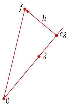
Here f=c g+h, where h is orthogonal to g.

8.10 orthogonal decomposition

Suppose f and g are elements of an inner product space, with g \neq 0. Then there exists h \in V such that

\langle h, g\rangle=0 \quad \text { and } \quad f=\frac{\langle f, g\rangle}{|g|^{2}} g+h

Proof Set h=f-\frac{\langle f, g\rangle}{\|g\|^{2}} g. Then

\langle h, g\rangle=\left\langle f-\frac{\langle f, g\rangle}{|g|^{2}} g, g\right\rangle=\langle f, g\rangle-\frac{\langle f, g\rangle}{|g|^{2}}\langle g, g\rangle=0

giving the first equation in the conclusion. The second equation in the conclusion follows immediately from the definition of h.

The orthogonal decomposition 8.10 is the main ingredient in our proof of the next result, which is one of the most important inequalities in mathematics.

8.11 Cauchy-Schwarz inequality

Suppose f and g are elements of an inner product space. Then

|\langle f, g\rangle| \leq|f||g|

with equality if and only if one of f, g is a scalar multiple of the other.

Proof If g=0, then both sides of the desired inequality equal 0 . Thus we can assume g \neq 0. Consider the orthogonal decomposition

f=\frac{\langle f, g\rangle}{|g|^{2}} g+h

given by 8.10 , where h is orthogonal to g. The Pythagorean Theorem (8.9) implies

\begin{aligned} |f|^{2} & =\left|\frac{\langle f, g\rangle}{|g|^{2}} g\right|^{2}+|h|^{2} \ & =\frac{|\langle f, g\rangle|^{2}}{|g|^{2}}+|h|^{2} \ & \geq \frac{|\langle f, g\rangle|^{2}}{|g|^{2}} . \end{aligned}

Multiplying both sides of this inequality by \|g\|^{2} and then taking square roots gives the desired inequality.

The proof above shows that the Cauchy-Schwarz inequality is an equality if and only if 8.12 is an equality. This happens if and only if h=0. But h=0 if and only if f is a scalar multiple of g (see 8.10). Thus the Cauchy-Schwarz inequality is an equality if and only if f is a scalar multiple of g or g is a scalar multiple of f (or both; the phrasing has been chosen to cover cases in which either f or g equals 0 ).

8.13 Example Cauchy-Schwarz inequality for \mathbf{F}^{n}

Applying the Cauchy-Schwarz inequality with the standard inner product on \mathbf{F}^{n} to \left(\left|a_{1}\right|, \ldots,\left|a_{n}\right|\right) and \left(\left|b_{1}\right|, \ldots,\left|b_{n}\right|\right) gives the inequality

\left|a_{1} b_{1}\right|+\cdots+\left|a_{n} b_{n}\right| \leq \sqrt{\left|a_{1}\right|^{2}+\cdots+\left|a_{n}\right|^{2}} \sqrt{\left|b_{1}\right|^{2}+\cdots+\left|b_{n}\right|^{2}}

for all \left(a_{1}, \ldots, a_{n}\right),\left(b_{1}, \ldots, b_{n}\right) \in \mathbf{F}^{n}.

Thus we have a new and clean proof of Hölder's inequality (7.9) for the special case where \mu is counting measure on

The inequality in this example was first proved by Cauchy in 1821. \{1, \ldots, n\} and p=p^{\prime}=2.

8.14 Example Cauchy-Schwarz inequality for L^{2}(\mu)

Suppose \mu is a measure and f, g \in L^{2}(\mu). Applying the Cauchy-Schwarz inequality with the standard inner product on L^{2}(\mu) to |f| and |g| gives the inequality

\int|f g| d \mu \leq\left(\int|f|^{2} d \mu\right)^{1 / 2}\left(\int|g|^{2} d \mu\right)^{1 / 2} .

The inequality above is equivalent to Hölder's inequality (7.9) for the special case where p=p^{\prime}=2. However, the proof of the inequality above via the Cauchy-Schwarz inequality still depends upon Hölder's inequality to show that the definition of the standard inner product on L^{2}(\mu) makes sense. See Exercise 18 in this section for a derivation of the in-

In 1859 Viktor Bunyakovsky (1804-1889), who had been Cauchy's student in Paris, first proved integral inequalities like the one above. Similar discoveries by Hermann Schwarz (1843-1921) in 1885 attracted more attention and led to the name of this inequality. equality above that is truly independent of Hölder's inequality.

If we think of the norm determined by an inner product as a length, then the triangle inequality has the geometric interpretation that the length of each side of a triangle is less than the sum of the lengths of the other two sides.

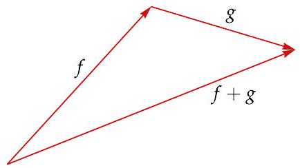
8.15 triangle inequality

Suppose f and g are elements of an inner product space. Then

|f+g| \leq|f|+|g|,

with equality if and only if one of f, g is a nonnegative multiple of the other.

Proof We have

\begin{aligned} |f+g|^{2} & =\langle f+g, f+g\rangle \ & =\langle f, f\rangle+\langle g, g\rangle+\langle f, g\rangle+\langle g, f\rangle \ & =\langle f, f\rangle+\langle g, g\rangle+\langle f, g\rangle+\overline{\langle f, g\rangle} \ & =|f|^{2}+|g|^{2}+2 \operatorname{Re}\langle f, g\rangle \end{aligned}

8.16

\leq|f|^{2}+|g|^{2}+2|\langle f, g\rangle|

8.17

\begin{aligned} & \leq|f|^{2}+|g|^{2}+2|f||g| \ & =(|f|+|g|)^{2} \end{aligned}

where 8.17 follows from the Cauchy-Schwarz inequality (8.11). Taking square roots of both sides of the inequality above gives the desired inequality.

The proof above shows that the triangle inequality is an equality if and only if we have equality in 8.16 and 8.17 . Thus we have equality in the triangle inequality if and only if

8.18

\langle f, g\rangle=|f||g| \text {. }

If one of f, g is a nonnegative multiple of the other, then 8.18 holds, as you should verify. Conversely, suppose 8.18 holds. Then the condition for equality in the CauchySchwarz inequality (8.11) implies that one of f, g is a scalar multiple of the other. Clearly 8.18 forces the scalar in question to be nonnegative, as desired.

Applying the previous result to the inner product space L^{2}(\mu), where \mu is a measure, gives a new proof of Minkowski's inequality (7.14) for the case p=2.

Now we can prove that what we have been calling a norm on an inner product space is indeed a norm.

8.19\|\cdot\| is a norm

Suppose V is an inner product space and \|f\| is defined as usual by

|f|=\sqrt{\langle f, f\rangle}

for f \in V. Then \|\cdot\| is a norm on V.

Proof The definition of an inner product implies that \|\cdot\| satisfies the positive definite requirement for a norm. The homogeneity and triangle inequality requirements for a norm are satisfied because of 8.6 and 8.15.

The next result has the geometric interpretation that the sum of the squares of the lengths of the diagonals of a parallelogram equals the sum of the squares of the lengths of the four sides.

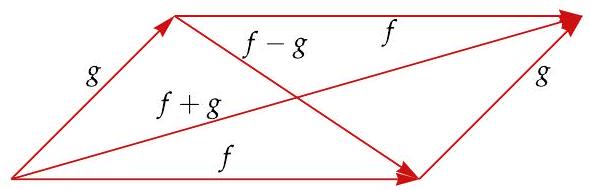
8.20 parallelogram equality

Suppose f and g are elements of an inner product space. Then

|f+g|^{2}+|f-g|^{2}=2|f|^{2}+2|g|^{2} .

Proof We have

\begin{aligned} |f+g|^{2}+|f-g|^{2}= & \langle f+g, f+g\rangle+\langle f-g, f-g\rangle \ = & |f|^{2}+|g|^{2}+\langle f, g\rangle+\langle g, f\rangle \ & +|f|^{2}+|g|^{2}-\langle f, g\rangle-\langle g, f\rangle \ = & 2|f|^{2}+2|g|^{2}, \end{aligned}

as desired.

EXERCISES 8A

1 Let V denote the vector space of bounded continuous functions from \mathbf{R} to \mathbf{F}. Let r_{1}, r_{2}, \ldots be a list of the rational numbers. For f, g \in V, define

\langle f, g\rangle=\sum_{k=1}^{\infty} \frac{f\left(r_{k}\right) \overline{g\left(r_{k}\right)}}{2^{k}}

Show that \langle\cdot, \cdot\rangle is an inner product on V.

2 Prove that if \mu is a measure and f, g \in L^{2}(\mu), then

|f|^{2}|g|^{2}-|\langle f, g\rangle|^{2}=\frac{1}{2} \iint|f(x) g(y)-g(x) f(y)|^{2} d \mu(y) d \mu(x) .

3 Suppose f and g are elements of an inner product space and

|f+g|^{2}=|f|^{2}+|g|^{2} \text {. }

(a) Prove that if \mathbf{F}=\mathbf{R}, then f and g are orthogonal.

(b) Give an example to show that if \mathbf{F}=\mathbf{C}, then f and g can satisfy the equation above without being orthogonal.

4 Find a, b \in \mathbf{R}^{3} such that a is a scalar multiple of (1,6,3), b is orthogonal to (1,6,3), and (5,4,-2)=a+b.

5 Prove that

16 \leq(a+b+c+d)\left(\frac{1}{a}+\frac{1}{b}+\frac{1}{c}+\frac{1}{d}\right)

for all positive numbers a, b, c, d, with equality if and only if a=b=c=d.

6 Prove that the square of the average of each finite list of real numbers containing at least two distinct real numbers is less than the average of the squares of the numbers in that list.

7 Suppose f and g are elements of an inner product space and \|f\| \leq 1 and \|g\| \leq 1. Prove that

\sqrt{1-|f|^{2}} \sqrt{1-|g|^{2}} \leq 1-|\langle f, g\rangle|

8 Suppose a and b are nonzero elements of \mathbf{R}^{2}. Prove that

\langle a, b\rangle=|a||b| \cos \theta,

where \theta is the angle between a and b (thinking of a as the vector whose initial point is the origin and whose end point is a, and similarly for b ).

Hint: Draw the triangle formed by a, b, and a-b; then use the law of cosines.

9 The angle between two vectors (thought of as arrows with initial point at the origin) in \mathbf{R}^{2} or \mathbf{R}^{3} can be defined geometrically. However, geometry is not as clear in \mathbf{R}^{n} for n>3. Thus the angle between two nonzero vectors a, b \in \mathbf{R}^{n} is defined to be

\arccos \frac{\langle a, b\rangle}{|a||b|}

where the motivation for this definition comes from the previous exercise. Explain why the Cauchy-Schwarz inequality is needed to show that this definition makes sense.

10 (a) Suppose f and g are elements of a real inner product space. Prove that f and g have the same norm if and only if f+g is orthogonal to f-g.

(b) Use part (a) to show that the diagonals of a parallelogram are perpendicular to each other if and only if the parallelogram is a rhombus.

11 Suppose f and g are elements of an inner product space. Prove that \|f\|=\|g\| if and only if \|s f+t g\|=\|t f+s g\| for all s, t \in \mathbf{R}.

12 Suppose f and g are elements of an inner product space and \|f\|=\|g\|=1 and \langle f, g\rangle=1. Prove that f=g.

13 Suppose f and g are elements of a real inner product space. Prove that

\langle f, g\rangle=\frac{|f+g|^{2}-|f-g|^{2}}{4}

14 Suppose f and g are elements of a complex inner product space. Prove that

\langle f, g\rangle=\frac{|f+g|^{2}-|f-g|^{2}+|f+i g|^{2} i-|f-i g|^{2} i}{4} .

15 Suppose f, g, h are elements of an inner product space. Prove that

\left|h-\frac{1}{2}(f+g)\right|^{2}=\frac{|h-f|^{2}+|h-g|^{2}}{2}-\frac{|f-g|^{2}}{4} \text {. }

16 Prove that a norm satisfying the parallelogram equality comes from an inner product. In other words, show that if V is a normed vector space whose norm \|\cdot\| satisfies the parallelogram equality, then there is an inner product \langle\cdot, \cdot\rangle on V such that \|f\|=\langle f, f\rangle^{1 / 2} for all f \in V.

17 Let \lambda denote Lebesgue measure on [1, \infty).

(a) Prove that if f:[1, \infty) \rightarrow[0, \infty) is Borel measurable, then

\left(\int_{1}^{\infty} f(x) d \lambda(x)\right)^{2} \leq \int_{1}^{\infty} x^{2}(f(x))^{2} d \lambda(x)

(b) Describe the set of Borel measurable functions f:[1, \infty) \rightarrow[0, \infty) such that the inequality in part (a) is an equality.

18 Suppose \mu is a measure. For f, g \in L^{2}(\mu), define \langle f, g\rangle by

\langle f, g\rangle=\int f \bar{g} d \mu

(a) Using the inequality

|f(x) \overline{g(x)}| \leq \frac{1}{2}\left(|f(x)|^{2}+|g(x)|^{2}\right)

verify that the integral above makes sense and the map sending f, g to \langle f, g\rangle defines an inner product on L^{2}(\mu) (without using Hölder's inequality).

(b) Show that the Cauchy-Schwarz inequality implies that

|f g|{1} \leq|f|{2}|g|_{2}

for all f, g \in L^{2}(\mu) (again, without using Hölder's inequality).

19 Suppose V_{1}, \ldots, V_{m} are inner product spaces. Show that the equation

\left\langle\left(f_{1}, \ldots, f_{m}\right),\left(g_{1}, \ldots, g_{m}\right)\right\rangle=\left\langle f_{1}, g_{1}\right\rangle+\cdots+\left\langle f_{m}, g_{m}\right\rangle

defines an inner product on V_{1} \times \cdots \times V_{m}.

[Each of the inner product spaces V_{1}, \ldots, V_{m} may have a different inner product, even though the same inner product notation is used on all these spaces.]

20 Suppose V is an inner product space. Make V \times V an inner product space as in the exercise above. Prove that the function that takes an ordered pair (f, g) \in V \times V to the inner product \langle f, g\rangle \in \mathbf{F} is a continuous function from V \times V to \mathbf{F}.

21 Suppose 1 \leq p \leq \infty.

(a) Show the norm on \ell^{p} comes from an inner product if and only if p=2.

(b) Show the norm on L^{p}(\mathbf{R}) comes from an inner product if and only if p=2.

22 Use inner products to prove Apollonius's identity: In a triangle with sides of length a, b, and c, let d be the length of the line segment from the midpoint of the side of length c to the opposite vertex. Then

a^{2}+b^{2}=\frac{1}{2} c^{2}+2 d^{2} .

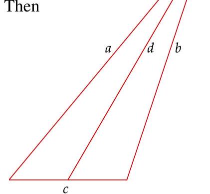
8B Orthogonality

Orthogonal Projections

The previous section developed inner product spaces following a standard linear algebra approach. Linear algebra focuses mainly on finite-dimensional vector spaces. Many interesting results about infinite-dimensional inner product spaces require an additional hypothesis, which we now introduce.

8.21 Definition Hilbert space

A Hilbert space is an inner product space that is a Banach space with the norm determined by the inner product.

8.22 Example Hilbert spaces

• Suppose \mu is a measure. Then L^{2}(\mu) with its usual inner product is a Hilbert space (by 7.24).
• As a special case of the first bullet point, if $n \in \mathbf{Z}^{+}$then taking \mu to be counting measure on \{1, \ldots, n\} shows that \mathbf{F}^{n} with its usual inner product is a Hilbert space.
• As another special case of the first bullet point, taking \mu to be counting measure on $\mathbf{Z}^{+}$shows that \ell^{2} with its usual inner product is a Hilbert space.
• Every closed subspace of a Hilbert space is a Hilbert space [by 6.16(b)].

8.23 Example not Hilbert spaces

• The inner product space \ell^{1}, where \left\langle\left(a_{1}, a_{2}, \ldots\right),\left(b_{1}, b_{2}, \ldots\right)\right\rangle=\sum_{k=1}^{\infty} a_{k} \overline{b_{k}}, is not a Hilbert space because the associated norm is not complete on \ell.
• The inner product space C([0,1]) of continuous $\mathbf{F}$-valued functions on the interval [0,1], where \langle f, g\rangle=\int_{0}^{1} f \bar{g}, is not a Hilbert space because the associated norm is not complete on C([0,1]).

The next definition makes sense in the context of normed vector spaces.

8.24 Definition distance from a point to a set

Suppose U is a nonempty subset of a normed vector space V and f \in V. The distance from f to U, denoted distance (f, U), is defined by

\text { distance }(f, U)=\inf {|f-g|: g \in U} \text {. }

Notice that distance (f, U)=0 if and only if f \in \bar{U}.

8.25 Definition convex

• A subset of a vector space is called convex if the subset contains the line segment connecting each pair of points in it.
• More precisely, suppose V is a vector space and U \subset V. Then U is called convex if

(1-t) f+t g \in U \text { for all } t \in[0,1] \text { and all } f, g \in U \text {. }

Convex subset of \mathbf{R}^{2}.

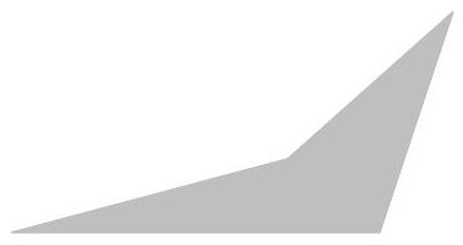
Nonconvex subset of \mathbf{R}^{2}.

8.26 Example convex sets

• Every subspace of a vector space is convex, as you should verify.
• If V is a normed vector space, f \in V, and r>0, then the open ball centered at f with radius r is convex, as you should verify.

The next example shows that the distance from an element of a Banach space to a closed subspace is not necessarily attained by some element of the closed subspace. After this example, we will prove that this behavior cannot happen in a Hilbert space.

8.27 Example no closest element to a closed subspace of a Banach space

In the Banach space C([0,1]) with norm \|g\|=\sup |g|, let

U=\left{g \in C([0,1]): \int_{0}^{1} g=0 \text { and } g(1)=0\right}

Then U is a closed subspace of C([0,1]).

Let f \in C([0,1]) be defined by f(x)=1-x. For k \in \mathbf{Z}^{+}, let

g_{k}(x)=\frac{1}{2}-x+\frac{x^{k}}{2}+\frac{x-1}{k+1}

Then g_{k} \in U and \lim _{k \rightarrow \infty}\left\|f-g_{k}\right\|=\frac{1}{2}, which implies that distance (f, U) \leq \frac{1}{2}.

If g \in U, then \int_{0}^{1}(f-g)=\frac{1}{2} and (f-g)(1)=0. These conditions imply that \|f-g\|>\frac{1}{2}.

Thus distance (f, U)=\frac{1}{2} but there does not exist g \in U such that \|f-g\|=\frac{1}{2}.

In the next result, we use for the first time the hypothesis that V is a Hilbert space.

8.28 distance to a closed convex set is attained in a Hilbert space

• The distance from an element of a Hilbert space to a nonempty closed convex set is attained by a unique element of the nonempty closed convex set.
• More specifically, suppose V is a Hilbert space, f \in V, and U is a nonempty closed convex subset of V. Then there exists a unique g \in U such that

|f-g|=\operatorname{distance}(f, U) \text {. }

Proof First we prove the existence of an element of U that attains the distance to f. To do this, suppose g_{1}, g_{2}, \ldots is a sequence of elements of U such that

8.29

\lim {k \rightarrow \infty}\left|f-g{k}\right|=\operatorname{distance}(f, U)

Then for $j, k \in \mathbf{Z}^{+}$we have

\begin{aligned} \left|g_{j}-g_{k}\right|^{2} & =\left|\left(f-g_{k}\right)-\left(f-g_{j}\right)\right|^{2} \ & =2\left|f-g_{k}\right|^{2}+2\left|f-g_{j}\right|^{2}-\left|2 f-\left(g_{k}+g_{j}\right)\right|^{2} \ & =2\left|f-g_{k}\right|^{2}+2\left|f-g_{j}\right|^{2}-4\left|f-\frac{g_{k}+g_{j}}{2}\right|^{2} \end{aligned}

8.30

\leq 2\left|f-g_{k}\right|^{2}+2\left|f-g_{j}\right|^{2}-4(\operatorname{distance}(f, U))^{2},

where the second equality comes from the parallelogram equality (8.20) and the last line holds because the convexity of U implies that \left(g_{k}+g_{j}\right) / 2 \in U. Now the inequality above and 8.29 imply that g_{1}, g_{2}, \ldots is a Cauchy sequence. Thus there exists g \in V such that

8.31

\lim {k \rightarrow \infty}\left|g{k}-g\right|=0

Because U is a closed subset of V and each g_{k} \in U, we know that g \in U. Now 8.29 and 8.31 imply that

|f-g|=\operatorname{distance}(f, U) \text {, }

which completes the existence proof of the existence part of this result.

To prove the uniqueness part of this result, suppose g and \widetilde{g} are elements of U such that

|f-g|=|f-\widetilde{g}|=\operatorname{distance}(f, U) \text {. }

Then

\begin{aligned} |g-\widetilde{g}|^{2} & \leq 2|f-g|^{2}+2|f-\widetilde{g}|^{2}-4(\text { distance }(f, U))^{2} \ & =0, \end{aligned}

where the first line above follows from 8.30 (with g_{j} replaced by g and g_{k} replaced by \widetilde{g} ) and the last line above follows from 8.32. Now 8.33 implies that g=\widetilde{g}, completing the proof of uniqueness.

Example 8.27 showed that the existence part of the previous result can fail in a Banach space. Exercise 13 shows that the uniqueness part can also fail in a Banach space. These observations highlight the advantages of working in a Hilbert space.

8.34 Definition orthogonal projection; P_{U}

Suppose U is a nonempty closed convex subset of a Hilbert space V. The orthogonal projection of V onto U is the function P_{U}: V \rightarrow V defined by setting P_{U}(f) equal to the unique element of U that is closest to f.

The definition above makes sense because of 8.28 . We will often use the notation P_{U} f instead of P_{U}(f). To test your understanding of the definition above, make sure that you can show that if U is a nonempty closed convex subset of a Hilbert space V, then

• P_{U} f=f if and only if f \in U;
• P_{U} \circ P_{U}=P_{U}.

8.35 Example orthogonal projection onto closed unit ball

Suppose U is the closed unit ball \{g \in V:\|g\| \leq 1\} in a Hilbert space V. Then

P_{U} f= \begin{cases}f & \text { if }|f| \leq 1 \ \frac{f}{|f|} & \text { if }|f|>1\end{cases}

as you should verify.

8.36 Example orthogonal projection onto a closed subspace

Suppose U is the closed subspace of \ell^{2} consisting of the elements of \ell^{2} whose even coordinates are all 0 :

U=\left{\left(a_{1}, 0, a_{3}, 0, a_{5}, 0, \ldots\right): \text { each } a_{k} \in \mathbf{F} \text { and } \sum_{k=1}^{\infty}\left|a_{2 k-1}\right|^{2}<\infty\right}

Then for b=\left(b_{1}, b_{2}, b_{3}, b_{4}, b_{5}, b_{6}, \ldots\right) \in \ell^{2}, we have

P_{U} b=\left(b_{1}, 0, b_{3}, 0, b_{5}, 0, \ldots\right),

as you should verify.

Note that in this example the function P_{U} is a linear map from \ell^{2} to \ell^{2} (unlike the behavior in Example 8.35).

Also, notice that b-P_{U} b=\left(0, b_{2}, 0, b_{4}, 0, b_{6}, \ldots\right) and thus b-P_{U} b is orthogonal to every element of U.

The next result shows that the properties stated in the last two paragraphs of the example above hold whenever U is a closed subspace of a Hilbert space.

8.37 orthogonal projection onto closed subspace

Suppose U is a closed subspace of a Hilbert space V and f \in V. Then

(a) f-P_{U} f is orthogonal to g for every g \in U;

(b) if h \in U and f-h is orthogonal to g for every g \in U, then h=P_{U} f;

(c) P_{U}: V \rightarrow V is a linear map;

(d) \left\|P_{U} f\right\| \leq\|f\|, with equality if and only if f \in U.

Proof The figure below illustrates (a). To prove (a), suppose g \in U. Then for all \alpha \in \mathbf{F} we have

\begin{aligned} \left|f-P_{U} f\right|^{2} & \leq\left|f-P_{U} f+\alpha g\right|^{2} \ & =\left\langle f-P_{U} f+\alpha g, f-P_{U} f+\alpha g\right\rangle \ & =\left|f-P_{U} f\right|^{2}+|\alpha|^{2}|g|^{2}+2 \operatorname{Re} \bar{\alpha}\left\langle f-P_{U} f, g\right\rangle . \end{aligned}

Let \alpha=-t\left\langle f-P_{U} f, g\right\rangle for t>0. A tiny bit of algebra applied to the inequality above implies

2\left|\left\langle f-P_{U} f, g\right\rangle\right|^{2} \leq t\left|\left\langle f-P_{U} f, g\right\rangle\right|^{2}|g|^{2}

for all t>0. Thus \left\langle f-P_{U} f, g\right\rangle=0, completing the proof of (a).

To prove (b), suppose h \in U and f-h is orthogonal to g for every g \in U. If g \in U, then h-g \in U and hence f-h is orthogonal to h-g. Thus

\begin{aligned} |f-h|^{2} & \leq|f-h|^{2}+|h-g|^{2} \ & =|(f-h)+(h-g)|^{2} \ & =|f-g|^{2}, \end{aligned}

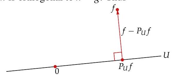
f-P_{U} f is orthogonal to each element of U.

where the first equality above follows from the Pythagorean Theorem (8.9). Thus

|f-h| \leq|f-g|

for all g \in U. Hence h is the element of U that minimizes the distance to f, which implies that h=P_{U} f, completing the proof of (b).

To prove (c), suppose f_{1}, f_{2} \in V. If g \in U, then (a) implies that \left\langle f_{1}-P_{U} f_{1}, g\right\rangle= \left\langle f_{2}-P_{U} f_{2}, g\right\rangle=0, and thus

\left\langle\left(f_{1}+f_{2}\right)-\left(P_{U} f_{1}+P_{U} f_{2}\right), g\right\rangle=0 .

The equation above and (b) now imply that

P_{U}\left(f_{1}+f_{2}\right)=P_{U} f_{1}+P_{U} f_{2} .

The equation above and the equation P_{U}(\alpha f)=\alpha P_{U} f for \alpha \in \mathbf{F} (whose proof is left to the reader) show that P_{U} is a linear map, proving (c).

The proof of (d) is left as an exercise for the reader.

Orthogonal Complements

8.38 Definition orthogonal complement; U^{\perp}

Suppose U is a subset of an inner product space V. The orthogonal complement of U is denoted by U^{\perp} and is defined by

U^{\perp}={h \in V:\langle g, h\rangle=0 \text { for all } g \in U}

In other words, the orthogonal complement of a subset U of an inner product space V is the set of elements of V that are orthogonal to every element of U.

8.39 Example orthogonal complement

Suppose U is the set of elements of \ell^{2} whose even coordinates are all 0 :

U=\left{\left(a_{1}, 0, a_{3}, 0, a_{5}, 0, \ldots\right): \text { each } a_{k} \in \mathbf{F} \text { and } \sum_{k=1}^{\infty}\left|a_{2 k-1}\right|^{2}<\infty\right}

Then U^{\perp} is the set of elements of \ell^{2} whose odd coordinates are all 0 :

as you should verify.

\left.U^{\perp}=\left{0, a_{2}, 0, a_{4}, 0, a_{6}, \ldots\right): \text { each } a_{k} \in \mathbf{F} \text { and } \sum_{k=1}^{\infty}\left|a_{2 k}\right|^{2}<\infty\right}

8.40 properties of orthogonal complement

Suppose U is a subset of an inner product space V. Then

(a) U^{\perp} is a closed subspace of V;

(b) U \cap U^{\perp} \subset\{0\};

(c) if W \subset U, then U^{\perp} \subset W^{\perp};

(d) \bar{U}^{\perp}=U^{\perp};

(e) U \subset\left(U^{\perp}\right)^{\perp}.

Proof To prove (a), suppose h_{1}, h_{2}, \ldots is a sequence in U^{\perp} that converges to some h \in V. If g \in U, then

|\langle g, h\rangle|=\left|\left\langle g, h-h_{k}\right\rangle\right| \leq|g|\left|h-h_{k}\right| \quad \text { for each } k \in \mathbf{Z}^{+} \text {; }

hence \langle g, h\rangle=0, which implies that h \in U^{\perp}. Thus U^{\perp} is closed. The proof of (a) is completed by showing that U^{\perp} is a subspace of V, which is left to the reader.

To prove (b), suppose g \in U \cap U^{\perp}. Then \langle g, g\rangle=0, which implies that g=0, proving (b).

To prove (e), suppose g \in U. Thus \langle g, h\rangle=0 for all h \in U^{\perp}, which implies that g \in\left(U^{\perp}\right)^{\perp}. Hence U \subset\left(U^{\perp}\right)^{\perp}, proving (e).

The proofs of (c) and (d) are left to the reader.

The results in the rest of this subsection have as a hypothesis that V is a Hilbert space. These results do not hold when V is only an inner product space.

8.41 orthogonal complement of the orthogonal complement

Suppose U is a subspace of a Hilbert space V. Then

\bar{U}=\left(U^{\perp}\right)^{\perp} .

Proof Applying 8.40(a) to U^{\perp}, we see that \left(U^{\perp}\right)^{\perp} is a closed subspace of V. Now taking closures of both sides of the inclusion U \subset\left(U^{\perp}\right)^{\perp} [8.40(e)] shows that \bar{U} \subset\left(U^{\perp}\right)^{\perp}.

To prove the inclusion in the other direction, suppose f \in\left(U^{\perp}\right)^{\perp}. Because f \in\left(U^{\perp}\right)^{\perp} and P_{\bar{U}} f \in \bar{U} \subset\left(U^{\perp}\right)^{\perp} (by the previous paragraph), we see that

f-P_{\bar{U}} f \in\left(U^{\perp}\right)^{\perp}

Also,

f-P_{\bar{U}} f \in U^{\perp}

by 8.37(a) and 8.40(d). Hence

f-P_{\bar{U}} f \in U^{\perp} \cap\left(U^{\perp}\right)^{\perp} .

Now 8.40(b) (applied to U^{\perp} in place of U ) implies that f-P_{\bar{U}} f=0, which implies that f \in \bar{U}. Thus \left(U^{\perp}\right)^{\perp} \subset \bar{U}, completing the proof.

As a special case, the result above implies that if U is a closed subspace of a Hilbert space V, then U=\left(U^{\perp}\right)^{\perp}.

Another special case of the result above is sufficiently useful to deserve stating separately, as we do in the next result.

8.42 necessary and sufficient condition for a subspace to be dense

Suppose U is a subspace of a Hilbert space V. Then

\bar{U}=V \text { if and only if } U^{\perp}={0}

Proof First suppose \bar{U}=V. Then using 8.40(\mathrm{~d}), we have

U^{\perp}=\bar{U}^{\perp}=V^{\perp}={0} .

To prove the other direction, now suppose U^{\perp}=\{0\}. Then 8.41 implies that

\bar{U}=\left(U^{\perp}\right)^{\perp}={0}^{\perp}=V

completing the proof.

The next result states that if U is a closed subspace of a Hilbert space V, then V is the direct sum of U and U^{\perp}, often written V=U \oplus U^{\perp}, although we do not need to use this terminology or notation further.

The key point to keep in mind is that the next result shows that the picture here represents what happens in general for a closed subspace U of a Hilbert space V : every element of V can be uniquely written as an element of U plus an element of U^{\perp}.

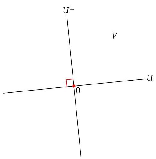
8.43 orthogonal decomposition

Suppose U is a closed subspace of a Hilbert space V. Then every element f \in V can be uniquely written in the form

f=g+h,

where g \in U and h \in U^{\perp}. Furthermore, g=P_{U} f and h=f-P_{U} f.

Proof Suppose f \in V. Then

f=P_{U} f+\left(f-P_{U} f\right)

where P_{U} f \in U [by definition of P_{U} f as the element of U that is closest to f ] and f-P_{U} f \in U^{\perp} [by 8.37(a)]. Thus we have the desired decomposition of f as the sum of an element of U and an element of U^{\perp}.

To prove the uniqueness of this decomposition, suppose

f=g_{1}+h_{1}=g_{2}+h_{2}

where g_{1}, g_{2} \in U and h_{1}, h_{2} \in U^{\perp}. Then g_{1}-g_{2}=h_{2}-h_{1} \in U \cap U^{\perp}, which implies that g_{1}=g_{2} and h_{1}=h_{2}, as desired.

In the next definition, the function I depends upon the vector space V. Thus a notation such as I_{V} might be more precise. However, the domain of I should always be clear from the context.

8.44 Definition identity map; I

Suppose V is a vector space. The identity map I is the linear map from V to V defined by I f=f for f \in V.

The next result highlights the close relationship between orthogonal projections and orthogonal complements.

8.45 range and null space of orthogonal projections

Suppose U is a closed subspace of a Hilbert space V. Then

(a) range P_{U}=U and null P_{U}=U^{\perp};

(b) range P_{U^{\perp}}=U^{\perp} and null P_{U^{\perp}}=U;

(c) P_{U^{\perp}}=I-P_{U}.

Proof The definition of P_{U} f as the closest point in U to f implies range P_{U} \subset U. Because P_{U} g=g for all g \in U, we also have U \subset range P_{U}. Thus range P_{U}=U.

If f \in null P_{U}, then f \in U^{\perp} [by 8.37(a)]. Thus null P_{U} \subset U^{\perp}. Conversely, if f \in U^{\perp}, then 8.37(b) (with h=0 ) implies that P_{U} f=0; hence U^{\perp} \subset null P_{U}. Thus null P_{U}=U^{\perp}, completing the proof of (a).

Replace U by U^{\perp} in (a), getting range P_{U^{\perp}}=U^{\perp} and null P_{U^{\perp}}=\left(U^{\perp}\right)^{\perp}=U (where the last equality comes from 8.41), completing the proof of (b).

Finally, if f \in U, then

P_{U^{\perp}} f=0=f-P_{U} f=\left(I-P_{U}\right) f

where the first equality above holds because null P_{U^{\perp}}=U [by (b)].

If f \in U^{\perp}, then

P_{U \perp} f=f=f-P_{U} f=\left(I-P_{U}\right) f,

where the second equality above holds because null P_{U}=U^{\perp} [by (a)].

The last two displayed equations show that P_{U^{\perp}} and I-P_{U} agree on U and agree on U^{\perp}. Because P_{U^{\perp}} and I-P_{U} are both linear maps and because each element of V equals some element of U plus some element of U^{\perp} (by 8.43), this implies that P_{U^{\perp}}=I-P_{U}, completing the proof of (c).

8.46 Example P_{U^{\perp}}=I-P_{U}

Suppose U is the closed subspace of L^{2}(\mathbf{R}) defined by

U=\left{f \in L^{2}(\mathbf{R}): f(x)=0 \text { for almost every } x<0\right} \text {. }

Then, as you should verify,

U^{\perp}=\left{g \in L^{2}(\mathbf{R}): g(x)=0 \text { for almost every } x \geq 0\right} \text {. }

Furthermore, you should also verify that if h \in L^{2}(\mathbf{R}), then

P_{U} h=h \chi_{[0, \infty)} \quad \text { and } \quad P_{U^{\perp}} h=h \chi_{(-\infty, 0)} .

Thus P_{U^{\perp}} h=h\left(1-\chi_{[0, \infty)}\right)=\left(I-P_{U}\right) h and hence P_{U^{\perp}}=I-P_{U}, as asserted in 8.45(c).

Riesz Representation Theorem

Suppose h is an element of a Hilbert space V. Define \varphi: V \rightarrow \mathbf{F} by \varphi(f)=\langle f, h\rangle for f \in V. The properties of an inner product imply that \varphi is a linear functional. The Cauchy-Schwarz inequality (8.11) implies that |\varphi(f)| \leq\|f\|\|h\| for all f \in V, which implies that \varphi is a bounded linear functional on V. The next result states that every bounded linear functional on V arises in this fashion.

To motivate the proof of the next result, note that if \varphi is as in the paragraph above, then null \varphi=\{h\}^{\perp}. Thus h \in(\text { null } \varphi)^{\perp} [by \left.8.40(\mathrm{e})\right]. Hence in the proof of the next result, to find h we start with an element of (\text { null } \varphi)^{\perp} and then multiply it by a scalar to make everything come out right.

8.47 Riesz Representation Theorem

Suppose \varphi is a bounded linear functional on a Hilbert space V. Then there exists a unique h \in V such that

\varphi(f)=\langle f, h\rangle

for all f \in V. Furthermore, \|\varphi\|=\|h\|.

Proof If \varphi=0, take h=0. Thus we can assume \varphi \neq 0. Hence null \varphi is a closed subspace of V not equal to V (see 6.52). The subspace (null \varphi)^{\perp} is not \{0\} (by 8.42). Thus there exists g \in(\text { null } \varphi)^{\perp} with \|g\|=1. Let

h=\overline{\varphi(g)} g

Taking the norm of both sides of the equation above, we get \|h\|=|\varphi(g)|. Thus

\varphi(h)=|\varphi(g)|^{2}=|h|^{2} .

Now suppose f \in V. Then

\begin{aligned} \langle f, h\rangle & =\left\langle f-\frac{\varphi(f)}{|h|^{2}} h, h\right\rangle+\left\langle\frac{\varphi(f)}{|h|^{2}} h, h\right\rangle \ & =\left\langle\frac{\varphi(f)}{|h|^{2}} h, h\right\rangle \ & =\varphi(f), \end{aligned}

where 8.49 holds because f-\frac{\varphi(f)}{\|h\|^{2}} h \in null \varphi (by 8.48) and h is orthogonal to all elements of null \varphi.

We have now proved the existence of h \in V such that \varphi(f)=\langle f, h\rangle for all f \in V. To prove uniqueness, suppose \widetilde{h} \in V has the same property. Then

\langle h-\widetilde{h}, h-\widetilde{h}\rangle=\langle h-\widetilde{h}, h\rangle-\langle h-\widetilde{h}, \widetilde{h}\rangle=\varphi(h-\widetilde{h})-\varphi(h-\widetilde{h})=0,

which implies that h=\widetilde{h}, which proves uniqueness.

The Cauchy-Schwarz inequality implies that |\varphi(f)|=|\langle f, h\rangle| \leq\|f\|\|h\| for all f \in V, which implies that \|\varphi\| \leq\|h\|. Because \varphi(h)=\langle h, h\rangle=\|h\|^{2}, we also have \|\varphi\| \geq\|h\|. Thus \|\varphi\|=\|h\|, completing the proof.

Suppose that \mu is a measure and 1<p \leq \infty. In 7.25 we considered the natural map of L^{p^{\prime}}(\mu) into \left(L^{p}(\mu)\right)^{\prime}, and

Frigyes Riesz (1880-1956) proved 8.47 in 1907. we showed that this maps preserves norms. In the special case where p=p^{\prime}=2, the Riesz Representation Theorem (8.47) shows that this map is surjective. In other words, if \varphi is a bounded linear functional on L^{2}(\mu), then there exists h \in L^{2}(\mu) such that

\varphi(f)=\int f h d \mu

for all f \in L^{2}(\mu) (take h to be the complex conjugate of the function given by 8.47). Hence we can identify the dual of L^{2}(\mu) with L^{2}(\mu). In 9.42 we will deal with other values of p. Also see Exercise 25 in this section.

EXERCISES 8B

1 Show that each of the inner product spaces in Example 8.23 is not a Hilbert space.

2 Prove or disprove: The inner product space in Exercise 1 in Section 8A is a Hilbert space.

3 Suppose V_{1}, V_{2}, \ldots are Hilbert spaces. Let

V=\left{\left(f_{1}, f_{2}, \ldots\right) \in V_{1} \times V_{2} \times \cdots: \sum_{k=1}^{\infty}\left|f_{k}\right|^{2}<\infty\right}

Show that the equation

\left\langle\left(f_{1}, f_{2}, \ldots\right),\left(g_{1}, g_{2}, \ldots\right)\right\rangle=\sum_{k=1}^{\infty}\left\langle f_{k}, g_{k}\right\rangle

defines an inner product on V that makes V a Hilbert space. [Each of the Hilbert spaces V_{1}, V_{2}, \ldots may have a different inner product, even though the same notation is used for the norm and inner product on all these Hilbert spaces.]

4 Suppose V is a real Hilbert space. The complexification of V is the complex vector space V_{\mathrm{C}} defined by V_{\mathrm{C}}=V \times V, but we write a typical element of V_{\mathrm{C}} as f+i g instead of (f, g). Addition and scalar multiplication are defined on V_{\mathrm{C}} by

\left(f_{1}+i g_{1}\right)+\left(f_{2}+i g_{2}\right)=\left(f_{1}+f_{2}\right)+i\left(g_{1}+g_{2}\right)

and

(\alpha+i \beta)(f+i g)=(\alpha f-\beta g)+i(\alpha g+\beta f)

for f_{1}, f_{2}, f, g_{1}, g_{2}, g \in V and \alpha, \beta \in \mathbf{R}. Show that

\left\langle f_{1}+i g_{1}, f_{2}+i g_{2}\right\rangle=\left\langle f_{1}, f_{2}\right\rangle+\left\langle g_{1}, g_{2}\right\rangle+i\left(\left\langle g_{1}, f_{2}\right\rangle-\left\langle f_{1}, g_{2}\right\rangle\right)

defines an inner product on V_{\mathbf{C}} that makes V_{\mathbf{C}} into a complex Hilbert space.

5 Prove that if V is a normed vector space, f \in V, and r>0, then the open ball B(f, r) centered at f with radius r is convex.

6 (a) Suppose V is an inner product space and B is the open unit ball in V (thus B=\{f \in V:\|f\|<1\} ). Prove that if U is a subset of V such that B \subset U \subset \bar{B}, then U is convex.

(b) Give an example to show that the result in part (a) can fail if the phrase inner product space is replaced by Banach space.

7 Suppose V is a normed vector space and U is a closed subset of V. Prove that U is convex if and only if

\frac{f+g}{2} \in U \text { for all } f, g \in U

8 Prove that if U is a convex subset of a normed vector space, then \bar{U} is also convex.

9 Prove that if U is a convex subset of a normed vector space, then the interior of U is also convex.

[The interior of U is the set \{f \in U: B(f, r) \subset U for some r>0\}.]

10 Suppose V is a Hilbert space, U is a nonempty closed convex subset of V, and g \in U is the unique element of U with smallest norm (obtained by taking f=0 in 8.28). Prove that

\operatorname{Re}\langle g, h\rangle \geq|g|^{2}

for all h \in U.

11 Suppose V is a Hilbert space. A closed half-space of V is a set of the form

{g \in V: \operatorname{Re}\langle g, h\rangle \geq c}

for some h \in V and some c \in \mathbf{R}. Prove that every closed convex subset of V is the intersection of all the closed half-spaces that contain it.

12 Give an example of a nonempty closed subset U of the Hilbert space \ell^{2} and a \in \ell^{2} such that there does not exist b \in U with \|a-b\|= distance (a, U). [By 8.28, U cannot be a convex subset of \ell^{2}.]

13 In the real Banach space \mathbf{R}^{2} with norm defined by \|(x, y)\|_{\infty}=\max \{|x|,|y|\}, give an example of a closed convex set U \subset \mathbf{R}^{2} and z \in \mathbf{R}^{2} such that there exist infinitely many choices of w \in U with \|z-w\|_{\infty}=\operatorname{distance}(z, U).

14 Suppose f and g are elements of an inner product space. Prove that \langle f, g\rangle=0 if and only if

|f| \leq|f+\alpha g|

for all \alpha \in \mathbf{F}.

15 Suppose U is a closed subspace of a Hilbert space V and f \in V. Prove that \left\|P_{U} f\right\| \leq\|f\|, with equality if and only if f \in U.

[This exercise asks you to prove 8.37(d).]

16 Suppose V is a Hilbert space and P: V \rightarrow V is a linear map such that P^{2}=P and \|P f\| \leq\|f\| for every f \in V. Prove that there exists a closed subspace U of V such that P=P_{U}.

17 Suppose U is a subspace of a Hilbert space V. Suppose also that W is a Banach space and S: U \rightarrow W is a bounded linear map. Prove that there exists a bounded linear map T: V \rightarrow W such that \left.T\right|_{U}=S and \|T\|=\|S\|.

[If W=\mathbf{F}, then this result is just the Hahn-Banach Theorem (6.69) for Hilbert spaces. The result here is stronger because it allows W to be an arbitrary Banach space instead of requiring W to be \mathbf{F}. Also, the proof in this Hilbert space context does not require use of Zorn's Lemma or the Axiom of Choice.]

18 Suppose U and W are subspaces of a Hilbert space V. Prove that \bar{U}=\bar{W} if and only if U^{\perp}=W^{\perp}.

19 Suppose U and W are closed subspaces of a Hilbert space. Prove that P_{U} P_{W}=0 if and only if \langle f, g\rangle=0 for all f \in U and all g \in W.

20 Verify the assertions in Example 8.46.

21 Show that every inner product space is a subspace of some Hilbert space.

Hint: See Exercise 13 in Section 6C.

22 Prove that if V is a Hilbert space and T: V \rightarrow V is a bounded linear map such that the dimension of range T is 1 , then there exist g, h \in V such that

T f=\langle f, g\rangle h

for all f \in V.

23 (a) Give an example of a Banach space V and a bounded linear functional \varphi on V such that |\varphi(f)|<\|\varphi\|\|f\| for all f \in V \backslash\{0\}.

(b) Show there does not exist an example in part (a) where V is a Hilbert space.

24 (a) Suppose \varphi and \psi are bounded linear functionals on a Hilbert space V such that \|\varphi+\psi\|=\|\varphi\|+\|\psi\|. Prove that one of \varphi, \psi is a scalar multiple of the other.

(b) Give an example to show that part (a) can fail if the hypothesis that V is a Hilbert space is replaced by the hypothesis that V is a Banach space.

25 (a) Suppose that \mu is a finite measure, 1 \leq p \leq 2, and \varphi is a bounded linear functional on L^{p}(\mu). Prove that there exists h \in L^{p^{\prime}}(\mu) such that \varphi(f)=\int f h d \mu for every f \in L^{p}(\mu).

(b) Same as part (a), but with the hypothesis that \mu is a finite measure replaced by the hypothesis that \mu is a measure, and assume that 1<p \leq 2.

[See 7.25, which along with this exercise shows that we can identify the dual of L^{p}(\mu) with L^{p^{\prime}}(\mu) for 1<p \leq 2. See 9.42 for an extension to all p \in(1, \infty).]

26 Prove that if V is an infinite-dimensional Hilbert space, then the Banach space \mathcal{B}(V, V) is nonseparable.

8 \mathrm{C} Orthonormal Bases

Bessel's Inequality

Recall that a family \left\{e_{k}\right\}_{k \in \Gamma} in a set V is a function e from a set \Gamma to V, with the value of the function e at k \in \Gamma denoted by e_{k} (see 6.53).

8.50 Definition orthonormal family

A family \left\{e_{k}\right\}_{k \in \Gamma} in an inner product space is called an orthonormal family if

\left\langle e_{j}, e_{k}\right\rangle= \begin{cases}0 & \text { if } j \neq k \ 1 & \text { if } j=k\end{cases}

for all j, k \in \Gamma.

In other words, a family \left\{e_{k}\right\}_{k \in \Gamma} is an orthonormal family if e_{j} and e_{k} are orthogonal for all distinct j, k \in \Gamma and \left\|e_{k}\right\|=1 for all k \in \Gamma.

8.51 Example orthonormal families

• For k \in \mathbf{Z}^{+}, let e_{k} be the element of \ell^{2} all of whose coordinates are 0 except for the k^{\text {th }} coordinate, which is 1 :

e_{k}=(0, \ldots, 0,1,0, \ldots)

Then $\left{e_{k}\right}{k \in \mathbf{Z}^{+}}$is an orthonormal family in \ell^{2}. In this case, our family is a sequence; thus we can call $\left{e{k}\right}_{k \in \mathbf{Z}^{+}}$an orthonormal sequence.

• More generally, suppose \Gamma is a nonempty set. The Hilbert space L^{2}(\mu), where \mu is counting measure on \Gamma, is often denoted by \ell^{2}(\Gamma). For k \in \Gamma, define a function e_{k}: \Gamma \rightarrow \mathbf{F} by

e_{k}(j)= \begin{cases}1 & \text { if } j=k \ 0 & \text { if } j \neq k\end{cases}

Then \left\{e_{k}\right\}_{k \in \Gamma} is an orthonormal family in \ell^{2}(\Gamma).

• For k \in \mathbf{Z}, define e_{k}:(-\pi, \pi] \rightarrow \mathbf{R} by

e_{k}(t)= \begin{cases}\frac{1}{\sqrt{\pi}} \sin (k t) & \text { if } k>0 \ \frac{1}{\sqrt{2 \pi}} & \text { if } k=0 \ \frac{1}{\sqrt{\pi}} \cos (k t) & \text { if } k<0\end{cases}

Then \left\{e_{k}\right\}_{k \in \mathbf{Z}} is an orthonormal family in L^{2}((-\pi, \pi]), as you should verify (see Exercise 1 for useful formulas that will help with this verification).

This orthonormal family \left\{e_{k}\right\}_{k \in \mathbf{Z}} leads to the classical theory of Fourier series, as we will see in more depth in Chapter 11.

• For k a nonnegative integer, define e_{k}:[0,1) \rightarrow \mathbf{F} by

e_{k}(x)= \begin{cases}1 & \text { if } x \in\left[\frac{n-1}{2^{k}}, \frac{n}{2^{k}}\right) \text { for some odd integer } n \ -1 & \text { if } x \in\left[\frac{n-1}{2^{k}}, \frac{n}{2^{k}}\right) \text { for some even integer } n\end{cases}

The figure below shows the graphs of e_{0}, e_{1}, e_{2}, and e_{3}. The pattern of these graphs should convince you that \left\{e_{k}\right\}_{k \in\{0,1, \ldots\}} is an orthonormal fam-

This orthonormal family was invented by Hans Rademacher (1892-1969). ily in L^{2}([0,1)).

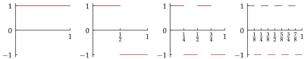
The graph of e_{0} . \quad The graph of e_{1}

The graph of e_{2}

The graph of e_{3}.

• Now we modify the example in the previous bullet point by translating the functions in the previous bullet point by arbitrary integers. Specifically, for k a nonnegative integer and m \in \mathbf{Z}, define e_{k, m}: \mathbf{R} \rightarrow \mathbf{F} by

e_{k, m}(x)= \begin{cases}1 & \text { if } x \in\left[m+\frac{n-1}{2^{k}}, m+\frac{n}{2^{k}}\right) \text { for some odd integer } n \in\left[1,2^{k}\right], \\ -1 & \text { if } x \in\left[m+\frac{n-1}{2^{k}}, m+\frac{n}{2^{k}}\right) \text { for some even integer } n \in\left[1,2^{k}\right], \\ 0 & \text { if } x \notin[m, m+1) .\end{cases}

Then \left\{e_{k, m}\right\}_{(k, m) \in\{0,1, \ldots\} \times \mathbf{Z}} is an orthonormal family in L^{2}(\mathbf{R}).

This example illustrates the usefulness of considering families that are not sequences. Although \{0,1, \ldots\} \times \mathbf{Z} is a countable set and hence we could rewrite \left\{e_{k, m}\right\}_{(k, m) \in\{0,1, \ldots\}} \times \mathbf{Z} as a sequence, doing so would be awkward and would be less clean than the e_{k, m} notation.

The next result gives our first indication of why orthonormal families are so useful.

8.52 finite orthonormal families

Suppose \Omega is a finite set and \left\{e_{j}\right\}_{j \in \Omega} is an orthonormal family in an inner product space. Then

\left|\sum_{j \in \Omega} \alpha_{j} e_{j}\right|^{2}=\sum_{j \in \Omega}\left|\alpha_{j}\right|^{2}

for every family \left\{\alpha_{j}\right\}_{j \in \Omega} in \mathbf{F}.

Proof Suppose \left\{\alpha_{j}\right\}_{j \in \Omega} is a family in F. Standard properties of inner products show that

\begin{aligned} \left|\sum_{j \in \Omega} \alpha_{j} e_{j}\right|^{2} & =\left\langle\sum_{j \in \Omega} \alpha_{j} e_{j}, \sum_{k \in \Omega} \alpha_{k} e_{k}\right\rangle \ & =\sum_{j, k \in \Omega} \alpha_{j} \overline{\alpha_{k}}\left\langle e_{j}, e_{k}\right\rangle \ & =\sum_{j \in \Omega}\left|\alpha_{j}\right|^{2}, \end{aligned}

as desired.

Suppose \Omega is a finite set and \left\{e_{j}\right\}_{j \in \Omega} is an orthonormal family in an inner product space. The result above implies that if \sum_{j \in \Omega} \alpha_{j} e_{j}=0, then \alpha_{j}=0 for every j \in \Omega.

Linear algebra, and algebra more generally, deals with sums of only finitely many terms. However, in analysis we often want to sum infinitely many terms. For example, earlier we defined the infinite sum of a sequence g_{1}, g_{2}, \ldots in a normed vector space to be the limit as n \rightarrow \infty of the partial sums \sum_{k=1}^{n} g_{k} if that limit exists (see 6.40).

The next definition captures a more powerful method of dealing with infinite sums. The sum defined below is called an unordered sum because the set \Gamma is not assumed to come with any ordering. A finite unordered sum is defined in the obvious way.

8.53 Definition unordered sum; \sum_{k \in \Gamma} f_{k}

Suppose \left\{f_{k}\right\}_{k \in \Gamma} is a family in a normed vector space V. The unordered sum \sum_{k \in \Gamma} f_{k} is said to converge if there exists g \in V such that for every \varepsilon>0, there exists a finite subset \Omega of \Gamma such that

\left|g-\sum_{j \in \Omega^{\prime}} f_{j}\right|<\varepsilon

for all finite sets \Omega^{\prime} with \Omega \subset \Omega^{\prime} \subset \Gamma. If this happens, we set \sum_{k \in \Gamma} f_{k}=g. If there is no such g \in V, then \sum_{k \in \Gamma} f_{k} is left undefined.

Exercises at the end of this section ask you to develop basic properties of unordered sums, including the following:

• Suppose \left\{a_{k}\right\}_{k \in \Gamma} is a family in \mathbf{R} and a_{k} \geq 0 for each k \in \Gamma. Then the unordered sum \sum_{k \in \Gamma} a_{k} converges if and only if

\sup \left{\sum_{j \in \Omega} a_{j}: \Omega \text { is a finite subset of } \Gamma\right}<\infty

Furthermore, if \sum_{k \in \Gamma} a_{k} converges then it equals the supremum above. If \sum_{k \in \Gamma} a_{k} does not converge, then the supremum above is \infty and we write \sum_{k \in \Gamma} a_{k}=\infty (this notation should be used only when a_{k} \geq 0 for each k \in \Gamma ).

• Suppose \left\{a_{k}\right\}_{k \in \Gamma} is a family in \mathbf{R}. Then the unordered sum \sum_{k \in \Gamma} a_{k} converges if and only if \sum_{k \in \Gamma}\left|a_{k}\right|<\infty. Thus convergence of an unordered summation in \mathbf{R} is the same as absolute convergence. As we are about to see, the situation in more general Hilbert spaces is quite different.

Now we can extend 8.52 to infinite sums.

8.54 linear combinations of an orthonormal family

Suppose \left\{e_{k}\right\}_{k \in \Gamma} is an orthonormal family in a Hilbert space V. Suppose \left\{\alpha_{k}\right\}_{k \in \Gamma} is a family in \mathbf{F}. Then

(a) the unordered sum \sum_{k \in \Gamma} \alpha_{k} e_{k} converges \Longleftrightarrow \sum_{k \in \Gamma}\left|\alpha_{k}\right|^{2}<\infty.

Furthermore, if \sum_{k \in \Gamma} \alpha_{k} e_{k} converges, then

(b)

\left|\sum_{k \in \Gamma} \alpha_{k} e_{k}\right|^{2}=\sum_{k \in \Gamma}\left|\alpha_{k}\right|^{2}

Proof First suppose \sum_{k \in \Gamma} \alpha_{k} e_{k} converges, with \sum_{k \in \Gamma} \alpha_{k} e_{k}=g. Suppose \varepsilon>0. Then there exists a finite set \Omega \subset \Gamma such that

\left|g-\sum_{j \in \Omega^{\prime}} \alpha_{j} e_{j}\right|<\varepsilon

for all finite sets \Omega^{\prime} with \Omega \subset \Omega^{\prime} \subset \Gamma. If \Omega^{\prime} is a finite set with \Omega \subset \Omega^{\prime} \subset \Gamma, then the inequality above implies that

|g|-\varepsilon<\left|\sum_{j \in \Omega^{\prime}} \alpha_{j} e_{j}\right|<|g|+\varepsilon

which (using 8.52) implies that

|g|-\varepsilon<\left(\sum_{j \in \Omega^{\prime}}\left|\alpha_{j}\right|^{2}\right)^{1 / 2}<|g|+\varepsilon

Thus \|g\|=\left(\sum_{k \in \Gamma}\left|\alpha_{k}\right|^{2}\right)^{1 / 2}, completing the proof of one direction of (a) and the proof of (b).

To prove the other direction of (a), now suppose \sum_{k \in \Gamma}\left|\alpha_{k}\right|^{2}<\infty. Thus there exists an increasing sequence \Omega_{1} \subset \Omega_{2} \subset \cdots of finite subsets of \Gamma such that for each m \in \mathbf{Z}^{+},

\sum_{j \in \Omega^{\prime} \backslash \Omega_{m}}\left|\alpha_{j}\right|^{2}<\frac{1}{m^{2}}

for every finite set \Omega^{\prime} such that \Omega_{m} \subset \Omega^{\prime} \subset \Gamma. For each m \in \mathbf{Z}^{+}, let

g_{m}=\sum_{j \in \Omega_{m}} \alpha_{j} e_{j} .

If n>m, then 8.52 implies that

\left|g_{n}-g_{m}\right|^{2}=\sum_{j \in \Omega_{n} \backslash \Omega_{m}}\left|\alpha_{j}\right|^{2}<\frac{1}{m^{2}}

Thus g_{1}, g_{2}, \ldots is a Cauchy sequence and hence converges to some element g of V.

Temporarily fixing $m \in \mathbf{Z}^{+}$and taking the limit of the equation above as n \rightarrow \infty, we see that

\left|g-g_{m}\right| \leq \frac{1}{m}

To show that \sum_{k \in \Gamma} \alpha_{k} e_{k}=g, suppose \varepsilon>0. Let $m \in \mathbf{Z}^{+}$be such that \frac{2}{m}<\varepsilon. Suppose \Omega^{\prime} is a finite set with \Omega_{m} \subset \Omega^{\prime} \subset \Gamma. Then

\begin{aligned} \left|g-\sum_{j \in \Omega^{\prime}} \alpha_{j} e_{j}\right| & \leq\left|g-g_{m}\right|+\left|g_{m}-\sum_{j \in \Omega^{\prime}} \alpha_{j} e_{j}\right| \ & \leq \frac{1}{m}+\left|\sum_{j \in \Omega^{\prime} \backslash \Omega_{m}} \alpha_{j} e_{j}\right| \ & =\frac{1}{m}+\left(\sum_{j \in \Omega^{\prime} \backslash \Omega_{m}}\left|\alpha_{j}\right|^{2}\right)^{1 / 2} \ & <\varepsilon, \end{aligned}

where the third line comes from 8.52 and the last line comes from 8.55 . Thus \sum_{k \in \Gamma} \alpha_{k} e_{k}=g, completing the proof.

8.56 Example a convergent unordered sum need not converge absolutely

Suppose $\left{e_{k}\right}_{k \in \mathbf{Z}^{+}}$is the orthogonal family in \ell^{2} defined by setting e_{k} equal to the sequence that is 0 everywhere except for a 1 in the k^{\text {th }} slot. Then by 8.54 , the unordered sum

\sum_{k \in \mathbf{Z}^{+}} \frac{1}{k} e_{k}

converges in \ell^{2} (because \sum_{k \in \mathbf{Z}^{+}} \frac{1}{k^{2}}<\infty ) even though \sum_{k \in \mathbf{Z}^{+}}\left\|\frac{1}{k} e_{k}\right\|=\infty. Note that \sum_{k \in \mathbf{Z}^{+}} \frac{1}{k} e_{k}=\left(1, \frac{1}{2}, \frac{1}{3}, \ldots\right) \in \ell^{2}.

Now we prove an important inequality.

8.57 Bessel's inequality

Suppose \left\{e_{k}\right\}_{k \in \Gamma} is an orthonormal family in an inner product space V and f \in V. Then

\sum_{k \in \Gamma}\left|\left\langle f, e_{k}\right\rangle\right|^{2} \leq|f|^{2}

Proof Suppose \Omega is a finite subset of \Gamma. Then

f=\sum_{j \in \Omega}\left\langle f, e_{j}\right\rangle e_{j}+\left(f-\sum_{j \in \Omega}\left\langle f, e_{j}\right\rangle e_{j}\right),

where the first sum above is orthogonal to the term in parentheses above (as you should verify).

Applying the Pythagorean Theorem (8.9) to the equation above gives

\begin{aligned} |f|^{2} & =\left|\sum_{j \in \Omega}\left\langle f, e_{j}\right\rangle e_{j}\right|^{2}+\left|f-\sum_{j \in \Omega}\left\langle f, e_{j}\right\rangle e_{j}\right|^{2} \ & \geq\left|\sum_{j \in \Omega}\left\langle f, e_{j}\right\rangle e_{j}\right|^{2} \ & =\sum_{j \in \Omega}\left|\left\langle f, e_{j}\right\rangle\right|^{2}, \end{aligned}

where the last equality follows from 8.52. Because the inequality above holds for every finite set \Omega \subset \Gamma, we conclude that \|f\|^{2} \geq \sum_{k \in \Gamma}\left|\left\langle f, e_{k}\right\rangle\right|^{2}, as desired.

Recall that the span of a family \left\{e_{k}\right\}_{k \in \Gamma} in a vector space is the set of finite sums of the form

\sum_{j \in \Omega} \alpha_{j} e_{j},

where \Omega is a finite subset of \Gamma and \left\{\alpha_{j}\right\}_{j \in \Omega} is a family in \mathbf{F} (see 6.54). Bessel's inequality now allows us to prove the following beautiful result showing that the closure of the span of an orthonormal family is a set of infinite sums.

8.58 closure of the span of an orthonormal family

Suppose \left\{e_{k}\right\}_{k \in \Gamma} is an orthonormal family in a Hilbert space V. Then

(a) \overline{\operatorname{span}\left\{e_{k}\right\}_{k \in \Gamma}}=\left\{\sum_{k \in \Gamma} \alpha_{k} e_{k}:\left\{\alpha_{k}\right\}_{k \in \Gamma}\right. is a family in \mathbf{F} and \left.\sum_{k \in \Gamma}\left|\alpha_{k}\right|^{2}<\infty\right\}.

Furthermore,

f=\sum_{k \in \Gamma}\left\langle f, e_{k}\right\rangle e_{k}

for every f \in \overline{\operatorname{span}\left\{e_{k}\right\}_{k \in \Gamma}}.

Proof The right side of (a) above makes sense because of 8.54(a). Furthermore, the right side of (a) above is a subspace of V because \ell^{2}(\Gamma) [which equals \mathcal{L}^{2}(\mu), where \mu is counting measure on \Gamma] is closed under addition and scalar multiplication by 7.5.

Suppose first \left\{\alpha_{k}\right\}_{k \in \Gamma} is a family in \mathbf{F} and \sum_{k \in \Gamma}\left|\alpha_{k}\right|^{2}<\infty. Let \varepsilon>0. Then there is a finite subset \Omega of \Gamma such that

\sum_{j \in \Gamma \backslash \Omega}\left|\alpha_{j}\right|^{2}<\varepsilon^{2}

The inequality above and 8.54 (b) imply that

\left|\sum_{k \in \Gamma} \alpha_{k} e_{k}-\sum_{j \in \Omega} \alpha_{j} e_{j}\right|<\varepsilon

The definition of the closure (see 6.7) now implies that \sum_{k \in \Gamma} \alpha_{k} e_{k} \in \overline{\operatorname{span}\left\{e_{k}\right\}_{k \in \Gamma}}, showing that the right side of (a) is contained in the left side of (a).

To prove the inclusion in the other direction, now suppose f \in \overline{\operatorname{span}\left\{e_{k}\right\}_{k \in \Gamma}}. Let

g=\sum_{k \in \Gamma}\left\langle f, e_{k}\right\rangle e_{k}

where the sum above converges by Bessel's inequality (8.57) and by 8.54(a). The direction of the inclusion that we just proved implies that g \in \overline{\operatorname{span}\left\{e_{k}\right\}_{k \in \Gamma}}. Thus

g-f \in \overline{\operatorname{span}\left{e_{k}\right}_{k \in \Gamma}} .

Equation 8.59 implies that \left\langle g, e_{j}\right\rangle=\left\langle f, e_{j}\right\rangle for each j \in \Gamma, as you should verify (which will require using the Cauchy-Schwarz inequality if done rigorously). Hence

\left\langle g-f, e_{k}\right\rangle=0 \quad \text { for every } k \in \Gamma .

This implies that

g-f \in\left(\operatorname{span}\left{e_{j}\right}{j \in \Gamma}\right)^{\perp}=\left(\overline{\operatorname{span}\left{e{j}\right}_{j \in \Gamma}}\right)^{\perp}

where the equality above comes from 8.40 (d). Now 8.60 and the inclusion above imply that f=g [see 8.40(\mathrm{~b}) ], which along with 8.59 implies that f is in the right side of (a), completing the proof of (a).

The equations f=g and 8.59 also imply (b).

Parseval's Identity

Note that 8.52 implies that every orthonormal family in an inner product space is linearly independent (see 6.54 to review the definition of linearly independent and basis). Linear algebra deals mainly with finite-dimensional vector spaces, but infinitedimensional vector spaces frequently appear in analysis. The notion of a basis is not so useful when doing analysis with infinite-dimensional vector spaces because the definition of span does not take advantage of the possibility of summing an infinite number of elements.

However, 8.58 tells us that taking the closure of the span of an orthonormal family can capture the sum of infinitely many elements. Thus we make the following definition.

8.61 Definition orthonormal basis

An orthonormal family \left\{e_{k}\right\}_{k \in \Gamma} in a Hilbert space V is called an orthonormal basis of V if

\overline{\operatorname{span}\left{e_{k}\right}_{k \in \Gamma}}=V .

In addition to requiring orthonormality (which implies linear independence), the definition above differs from the definition of a basis by considering the closure of the span rather than the span. An important point to keep in mind is that despite the terminology, an orthonormal basis is not necessarily a basis in the sense of 6.54. In fact, if \Gamma is an infinite set and \left\{e_{k}\right\}_{k \in \Gamma} is an orthonormal basis of V, then \left\{e_{k}\right\}_{k \in \Gamma} is not a basis of V (see Exercise 9).

8.62 Example orthonormal bases

• For $n \in \mathbf{Z}^{+}$and k \in\{1, \ldots, n\}, let e_{k} be the element of \mathbf{F}^{n} all of whose coordinates are 0 except the k^{\text {th }} coordinate, which is 1 :

e_{k}=(0, \ldots, 0,1,0, \ldots, 0) .

Then \left\{e_{k}\right\}_{k \in\{1, \ldots, n\}} is an orthonormal basis of \mathbf{F}^{n}.

• Let e_{1}=\left(\frac{1}{\sqrt{3}}, \frac{1}{\sqrt{3}}, \frac{1}{\sqrt{3}}\right), e_{2}=\left(-\frac{1}{\sqrt{2}}, \frac{1}{\sqrt{2}}, 0\right), and e_{3}=\left(\frac{1}{\sqrt{6}}, \frac{1}{\sqrt{6}},-\frac{2}{\sqrt{6}}\right). Then \left\{e_{k}\right\}_{k \in\{1,2,3\}} is an orthonormal basis of \mathbf{F}^{3}, as you should verify.
• The first three bullet points in 8.51 are examples of orthonormal families that are orthonormal bases. The exercises ask you to verify that we have an orthonormal basis in the first and second bullet points of 8.51. For the third bullet point (trigonometric functions), see Exercise 11 in Section 10D or see Chapter 11.

The next result shows why orthonormal bases are so useful—a Hilbert space with an orthonormal basis \left\{e_{k}\right\}_{k \in \Gamma} behaves like \ell^{2}(\Gamma).

8.63 Parseval's identity

Suppose \left\{e_{k}\right\}_{k \in \Gamma} is an orthonormal basis of a Hilbert space V and f, g \in V. Then

(a) f=\sum_{k \in \Gamma}\left\langle f, e_{k}\right\rangle e_{k}

(b) \langle f, g\rangle=\sum_{k \in \Gamma}\left\langle f, e_{k}\right\rangle \overline{\left\langle g, e_{k}\right\rangle};

(c) \|f\|^{2}=\sum_{k \in \Gamma}\left|\left\langle f, e_{k}\right\rangle\right|^{2}.

Proof The equation in (a) follows immediately from 8.58(b) and the definition of an orthonormal basis.

To prove (b), note that

\begin{aligned} \langle f, g\rangle & =\left\langle\sum_{k \in \Gamma}\left\langle f, e_{k}\right\rangle e_{k}, g\right\rangle \ & =\sum_{k \in \Gamma}\left\langle f, e_{k}\right\rangle\left\langle e_{k}, g\right\rangle \ & =\sum_{k \in \Gamma}\left\langle f, e_{k}\right\rangle \overline{\left\langle g, e_{k}\right\rangle}, \end{aligned}

Equation (c) is called Parseval's identity in honor of Marc-Antoine Parseval (1755-1836), who discovered a special case in 1799.

where the first equation follows from (a) and the second equation follows from the definition of an unordered sum and the Cauchy-Schwarz inequality.

Equation (c) follows from setting g=f in (b). An alternative proof: equation (c) follows from 8.54(b) and the equation f=\sum_{k \in \Gamma}\left\langle f, e_{k}\right\rangle e_{k} from (a).

Gram-Schmidt Process and Existence of Orthonormal Bases

8.64 Definition separable

A normed vector space is called separable if it has a countable subset whose closure equals the whole space.

8.65 Example separable normed vector spaces

• Suppose n \in \mathbf{Z}^{+}. Then \mathbf{F}^{n} with the usual Hilbert space norm is separable because the closure of the countable set

\left{\left(c_{1}, \ldots, c_{n}\right) \in \mathbf{F}^{n}: \text { each } c_{j} \text { is rational }\right}

equals \mathbf{F}^{n} (in case \mathbf{F}=\mathbf{C} : to say that a complex number is rational in this context means that both the real and imaginary parts of the complex number are rational numbers in the usual sense).

• The Hilbert space \ell^{2} is separable because the closure of the countable set

\bigcup_{n=1}^{\infty}\left{\left(c_{1}, \ldots, c_{n}, 0,0, \ldots\right) \in \ell^{2}: \text { each } c_{j} \text { is rational }\right}

is \ell^{2}.

• The Hilbert spaces L^{2}([0,1]) and L^{2}(\mathbf{R}) are separable, as Exercise 13 asks you to verify [hint: consider finite linear combinations with rational coefficients of functions of the form \chi_{(c, d)}, where c and d are rational numbers].

A moment's thought about the definition of closure (see 6.7) shows that a normed vector space V is separable if and only if there exists a countable subset C of V such that every open ball in V contains at least one element of C.

8.66 Example nonseparable normed vector spaces

• Suppose \Gamma is an uncountable set. Then the Hilbert space \ell^{2}(\Gamma) is not separable. To see this, note that \left\|\chi_{\{j\}}-\chi_{\{k\}}\right\|=\sqrt{2} for all j, k \in \Gamma with j \neq k. Hence

\left{B\left(\chi_{{k}}, \frac{\sqrt{2}}{2}\right): k \in \Gamma\right}

is an uncountable collection of disjoint open balls in \ell^{2}(\Gamma); no countable set can have at least one element in each of these balls.

• The Banach space L^{\infty}([0,1]) is not separable. Here \left\|\chi_{[0, s]}-\chi_{[0, t]}\right\|=1 for all s, t \in[0,1] with s \neq t. Thus

\left{B\left(\chi_{[0, t]}, \frac{1}{2}\right): t \in[0,1]\right}

is an uncountable collection of disjoint open balls in L^{\infty}([0,1]).

We present two proofs of the existence of orthonormal bases of Hilbert spaces. The first proof works only for separable Hilbert spaces, but it gives a useful algorithm, called the Gram-Schmidt process, for constructing orthonormal sequences. The second proof works for all Hilbert spaces, but it uses a result that depends upon the Axiom of Choice.

Which proof should you read? In practice, the Hilbert spaces you will encounter will almost certainly be separable. Thus the first proof suffices, and it has the additional benefit of introducing you to a widely used algorithm. The second proof uses an entirely different approach and has the advantage of applying to separable and nonseparable Hilbert spaces. For maximum learning, read both proofs!

8.67 existence of orthonormal bases for separable Hilbert spaces

Every separable Hilbert space has an orthonormal basis.

Proof Suppose V is a separable Hilbert space and \left\{f_{1}, f_{2}, \ldots\right\} is a countable subset of V whose closure equals V. We will inductively define an orthonormal sequence $\left{e_{k}\right}_{k \in \mathbf{Z}^{+}}$such that

\operatorname{span}\left{f_{1}, \ldots, f_{n}\right} \subset \operatorname{span}\left{e_{1}, \ldots, e_{n}\right}

for each n \in \mathbf{Z}^{+}. This will imply that \overline{\operatorname{span}\left\{e_{k}\right\}_{k \in \mathbf{Z}^{+}}}=V, which will mean that $\left{e_{k}\right}_{k \in \mathbf{Z}^{+}}$is an orthonormal basis of V.

To get started with the induction, set e_{1}=f_{1} /\left\|f_{1}\right\| (we can assume that f_{1} \neq 0 ).

Now suppose $n \in \mathbf{Z}^{+}$and e_{1}, \ldots, e_{n} have been chosen so that \left\{e_{k}\right\}_{k \in\{1, \ldots, n\}} is an orthonormal family in V and 8.68 holds. If f_{k} \in \operatorname{span}\left\{e_{1}, \ldots, e_{n}\right\} for every k \in \mathbf{Z}^{+}, then \left\{e_{k}\right\}_{k \in\{1, \ldots, n\}} is an orthonormal basis of V (completing the proof) and the process should be stopped. Otherwise, let m be the smallest positive integer such that

8.69

f_{m} \notin \operatorname{span}\left{e_{1}, \ldots, e_{n}\right} .

Define e_{n+1} by

8.70

e_{n+1}=\frac{f_{m}-\left\langle f_{m}, e_{1}\right\rangle e_{1}-\cdots-\left\langle f_{m}, e_{n}\right\rangle e_{n}}{\left|f_{m}-\left\langle f_{m}, e_{1}\right\rangle e_{1}-\cdots-\left\langle f_{m}, e_{n}\right\rangle e_{n}\right|}

Clearly \left\|e_{n+1}\right\|=1 (8.69 guarantees there is no division by 0 ). If k \in\{1, \ldots, n\}, then the equation above implies that \left\langle e_{n+1}, e_{k}\right\rangle=0. Thus \left\{e_{k}\right\}_{k \in\{1, \ldots, n+1\}} is an orthonormal fam-

Jørgen Gram (1850-1916) and Erhard Schmidt (1876-1959) popularized this process that constructs orthonormal sequences. ily in V. Also, 8.68 and the choice of m as the smallest positive integer satisfying 8.69 imply that

\operatorname{span}\left{f_{1}, \ldots, f_{n+1}\right} \subset \operatorname{span}\left{e_{1}, \ldots, e_{n+1}\right}

completing the induction and completing the proof.

Before considering nonseparable Hilbert spaces, we take a short detour to illustrate how the Gram-Schmidt process used in the previous proof can be used to find closest elements to subspaces. We begin with a result connecting the orthogonal projection onto a closed subspace with an orthonormal basis of that subspace.

8.71 orthogonal projection in terms of an orthonormal basis

Suppose that U is a closed subspace of a Hilbert space V and \left\{e_{k}\right\}_{k \in \Gamma} is an orthonormal basis of U. Then

P_{U} f=\sum_{k \in \Gamma}\left\langle f, e_{k}\right\rangle e_{k}

for all f \in V.

Proof Let f \in V. If k \in \Gamma, then

8.72

\left\langle f, e_{k}\right\rangle=\left\langle f-P_{U} f, e_{k}\right\rangle+\left\langle P_{U} f, e_{k}\right\rangle=\left\langle P_{U} f, e_{k}\right\rangle,

where the last equality follows from 8.37 (a). Now

P_{U} f=\sum_{k \in \Gamma}\left\langle P_{U} f, e_{k}\right\rangle e_{k}=\sum_{k \in \Gamma}\left\langle f, e_{k}\right\rangle e_{k},

where the first equality follows from Parseval's identity [8.63(a)] as applied to U and its orthonormal basis \left\{e_{k}\right\}_{k \in \Gamma}, and the second equality follows from 8.72.

8.73 Example best approximation

Find the polynomial g of degree at most 10 that minimizes

\int_{-1}^{1}|\sqrt{|x|}-g(x)|^{2} d x

Solution We will work in the real Hilbert space L^{2}([-1,1]) with the usual inner product \langle g, h\rangle=\int_{-1}^{1} g h. For k \in\{0,1, \ldots, 10\}, let f_{k} \in L^{2}([-1,1]) be defined by f_{k}(x)=x^{k}. Let U be the subspace of L^{2}([-1,1]) defined by

U=\operatorname{span}\left{f_{k}\right}_{k \in{0, \ldots, 10}}

Apply the Gram-Schmidt process from the proof of 8.67 to \left\{f_{k}\right\}_{k \in\{0, \ldots, 10\}}, producing an orthonormal basis \left\{e_{k}\right\}_{k \in\{0, \ldots, 10\}} of U, which is a closed subspace of L^{2}([-1,1]) (see Exercise 8). The point here is that \left\{e_{k}\right\}_{k \in\{0, \ldots, 10\}} can be computed explicitly and exactly by using 8.70 and evaluating some integrals (using software that can do exact rational arithmetic will make the process easier), getting e_{0}(x)=1 / \sqrt{2}, e_{1}(x)=\sqrt{6} x / 2, \ldots up to

e_{10}(x)=\frac{\sqrt{42}}{512}\left(-63+3465 x^{2}-30030 x^{4}+90090 x^{6}-109395 x^{8}+46189 x^{10}\right).

Define f \in L^{2}([-1,1]) by f(x)=\sqrt{|x|}. Because U is the subspace of L^{2}([-1,1]) consisting of polynomials of degree at most 10 and P_{U} f equals the element of U closest to f (see 8.34), the formula in 8.71 tells us that the solution g to our minimization problem is given by the formula

g=\sum_{k=0}^{10}\left\langle f, e_{k}\right\rangle e_{k}

Using the explicit expressions for e_{0}, \ldots, e_{10} and again evaluating some integrals, this gives

g(x)=\frac{693+15015 x^{2}-64350 x^{4}+139230 x^{6}-138567 x^{8}+51051 x^{10}}{2944} .

The figure here shows the graph of f(x)=\sqrt{|x|} (red) and the graph of its closest polynomial g (blue) of degree at most 10 ; here closest means as measured in the norm of L^{2}([-1,1]).

The approximation of f by g is pretty good, especially considering that f is not differentiable at 0 and thus a Taylor series expansion for f does not make sense.

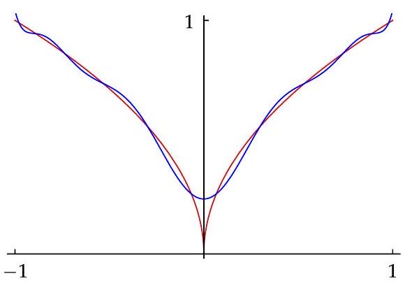
Recall that a subset \Gamma of a set V can be thought of as a family in V by considering \left\{e_{f}\right\}_{f \in \Gamma}, where e_{f}=f. With this convention, a subset \Gamma of an inner product space V is an orthonormal subset of V if \|f\|=1 for all f \in \Gamma and \langle f, g\rangle=0 for all f, g \in \Gamma with f \neq g.

The next result characterizes the orthonormal bases as the maximal elements among the collection of orthonormal subsets of a Hilbert space. Recall that a set \Gamma \in \mathcal{A} in a collection of subsets of a set V is a maximal element of \mathcal{A} if there does not exist \Gamma^{\prime} \in \mathcal{A} such that \Gamma \varsubsetneqq \Gamma^{\prime} (see 6.55).

8.74 orthonormal bases as maximal elements

Suppose V is a Hilbert space, \mathcal{A} is the collection of all orthonormal subsets of V, and \Gamma is an orthonormal subset of V. Then \Gamma is an orthonormal basis of V if and only if \Gamma is a maximal element of \mathcal{A}.

Proof First suppose \Gamma is an orthonormal basis of V. Parseval's identity [8.63(a)] implies that the only element of V that is orthogonal to every element of \Gamma is 0 . Thus there does not exist an orthonormal subset of V that strictly contains \Gamma. In other words, \Gamma is a maximal element of \mathcal{A}.

To prove the other direction, suppose now that \Gamma is a maximal element of \mathcal{A}. Let U denote the span of \Gamma. Then

U^{\perp}={0}

because if f is a nonzero element of U^{\perp}, then \Gamma \cup\{f /\|f\|\} is an orthonormal subset of V that strictly contains \Gamma. Hence \bar{U}=V (by 8.42), which implies that \Gamma is an orthonormal basis of V.

Now we are ready to prove that every Hilbert space has an orthonormal basis. Before reading the next proof, you may want to review the definition of a chain (6.58), which is a collection of sets such that for each pair of sets in the collection, one of them is contained in the other. You should also review Zorn's Lemma (6.60), which gives a way to show that a collection of sets contains a maximal element.

8.75 existence of orthonormal bases for all Hilbert spaces

Every Hilbert space has an orthonormal basis.

Proof Suppose V is a Hilbert space. Let \mathcal{A} be the collection of all orthonormal subsets of V. Suppose \mathcal{C} \subset \mathcal{A} is a chain. Let L be the union of all the sets in \mathcal{C}. If f \in L, then \|f\|=1 because f is an element of some orthonormal subset of V that is contained in \mathcal{C}.

If f, g \in L with f \neq g, then there exist orthonormal subsets \Omega and \Gamma in \mathcal{C} such that f \in \Omega and g \in \Gamma. Because \mathcal{C} is a chain, either \Omega \subset \Gamma or \Gamma \subset \Omega. Either way, there is an orthonormal subset of V that contains both f and g. Thus \langle f, g\rangle=0.

We have shown that L is an orthonormal subset of V; in other words, L \in \mathcal{A}. Thus Zorn's Lemma (6.60) implies that \mathcal{A} has a maximal element. Now 8.74 implies that V has an orthonormal basis.

Riesz Representation Theorem, Revisited

Now that we know that every Hilbert space has an orthonormal basis, we can give a completely different proof of the Riesz Representation Theorem (8.47) than the proof we gave earlier.

Note that the new proof below of the Riesz Representation Theorem gives the formula 8.77 for h in terms of an orthonormal basis. One interesting feature of this formula is that h is uniquely determined by \varphi and thus h does not depend upon the choice of an orthonormal basis. Hence despite its appearance, the right side of 8.77 is independent of the choice of an orthonormal basis.

8.76 Riesz Representation Theorem

Suppose \varphi is a bounded linear functional on a Hilbert space V and \left\{e_{k}\right\}_{k \in \Gamma} is an orthonormal basis of V. Let

8.77

h=\sum_{k \in \Gamma} \overline{\varphi\left(e_{k}\right)} e_{k}

Then

8.78

\varphi(f)=\langle f, h\rangle

for all f \in V. Furthermore, \|\varphi\|=\left(\sum_{k \in \Gamma}\left|\varphi\left(e_{k}\right)\right|^{2}\right)^{1 / 2}.

Proof First we must show that the sum defining h makes sense. To do this, suppose \Omega is a finite subset of \Gamma. Then

\sum_{j \in \Omega}\left|\varphi\left(e_{j}\right)\right|^{2}=\varphi\left(\sum_{j \in \Omega} \overline{\varphi\left(e_{j}\right)} e_{j}\right) \leq|\varphi|\left|\sum_{j \in \Omega} \overline{\varphi\left(e_{j}\right)} e_{j}\right|=|\varphi|\left(\sum_{j \in \Omega}\left|\varphi\left(e_{j}\right)\right|^{2}\right)^{1 / 2},

where the last equality follows from 8.52. Dividing by \left(\sum_{j \in \Omega}\left|\varphi\left(e_{j}\right)\right|^{2}\right)^{1 / 2} gives

\left(\sum_{j \in \Omega}\left|\varphi\left(e_{j}\right)\right|^{2}\right)^{1 / 2} \leq|\varphi|

Because the inequality above holds for every finite subset \Omega of \Gamma, we conclude that

\sum_{k \in \Gamma}\left|\varphi\left(e_{k}\right)\right|^{2} \leq|\varphi|^{2}

Thus the sum defining h makes sense (by 8.54) in equation 8.77.

Now 8.77 shows that \left\langle h, e_{j}\right\rangle=\overline{\varphi\left(e_{j}\right)} for each j \in \Gamma. Thus if f \in V then

\varphi(f)=\varphi\left(\sum_{k \in \Gamma}\left\langle f, e_{k}\right\rangle e_{k}\right)=\sum_{k \in \Gamma}\left\langle f, e_{k}\right\rangle \varphi\left(e_{k}\right)=\sum_{k \in \Gamma}\left\langle f, e_{k}\right\rangle \overline{\left\langle h, e_{k}\right\rangle}=\langle f, h\rangle,

where the first and last equalities follow from 8.63 and the second equality follows from the boundedness/continuity of \varphi. Thus 8.78 holds.

Finally, the Cauchy-Schwarz inequality, equation 8.78 , and the equation \varphi(h)= \langle h, h\rangle show that \|\varphi\|=\|h\|=\left(\sum_{k \in \Gamma}\left|\varphi\left(e_{k}\right)\right|^{2}\right)^{1 / 2}.

EXERCISES 8C

1 Verify that the family \left\{e_{k}\right\}_{k \in \mathbf{Z}} as defined in the third bullet point of Example 8.51 is an orthonormal family in L^{2}((-\pi, \pi]). The following formulas should help:

\begin{aligned} & (\sin x)(\cos y)=\frac{\sin (x-y)+\sin (x+y)}{2}, \ & (\sin x)(\sin y)=\frac{\cos (x-y)-\cos (x+y)}{2}, \ & (\cos x)(\cos y)=\frac{\cos (x-y)+\cos (x+y)}{2} . \end{aligned}

2 Suppose \left\{a_{k}\right\}_{k \in \Gamma} is a family in \mathbf{R} and a_{k} \geq 0 for each k \in \Gamma. Prove the unordered sum \sum_{k \in \Gamma} a_{k} converges if and only if

\sup \left{\sum_{j \in \Omega} a_{j}: \Omega \text { is a finite subset of } \Gamma\right}<\infty

Furthermore, prove that if \sum_{k \in \Gamma} a_{k} converges then it equals the supremum above.

3 Suppose \left\{e_{k}\right\}_{k \in \Gamma} is an orthonormal family in an inner product space V. Prove that if f \in V, then \left\{k \in \Gamma:\left\langle f, e_{k}\right\rangle \neq 0\right\} is a countable set.

4 Suppose \left\{f_{k}\right\}_{k \in \Gamma} and \left\{g_{k}\right\}_{k \in \Gamma} are families in a normed vector space such that \sum_{k \in \Gamma} f_{k} and \sum_{k \in \Gamma} g_{k} converge. Prove that \sum_{k \in \Gamma}\left(f_{k}+g_{k}\right) converges and

\sum_{k \in \Gamma}\left(f_{k}+g_{k}\right)=\sum_{k \in \Gamma} f_{k}+\sum_{k \in \Gamma} g_{k}

5 Suppose \left\{f_{k}\right\}_{k \in \Gamma} is a family in a normed vector space such that \sum_{k \in \Gamma} f_{k} converges. Prove that if c \in \mathbf{F}, then \sum_{k \in \Gamma}\left(c f_{k}\right) converges and

\sum_{k \in \Gamma}\left(c f_{k}\right)=c \sum_{k \in \Gamma} f_{k}

6 Suppose \left\{a_{k}\right\}_{k \in \Gamma} is a family in \mathbf{R}. Prove that the unordered sum \sum_{k \in \Gamma} a_{k} converges if and only if \sum_{k \in \Gamma}\left|a_{k}\right|<\infty.

7 Suppose $\left{f_{k}\right}_{k \in \mathbf{Z}^{+}}$is a family in a normed vector space V and f \in V. Prove that the unordered sum \sum_{k \in \mathbf{Z}^{+}} f_{k} equals f if and only if the usual ordered sum \sum_{k=1}^{\infty} f_{p(k)} equals f for every injective and surjective function p: \mathbf{Z}^{+} \rightarrow \mathbf{Z}^{+}.

8 Explain why 8.58 implies that if \Gamma is a finite set and \left\{e_{k}\right\}_{k \in \Gamma} is an orthonormal family in a Hilbert space V, then \operatorname{span}\left\{e_{k}\right\}_{k \in \Gamma} is a closed subspace of V.

9 Suppose V is an infinite-dimensional Hilbert space. Prove that there does not exist a basis of V that is an orthonormal family.

10 (a) Show that the orthonormal family given in the first bullet point of Example 8.51 is an orthonormal basis of \ell^{2}.

(b) Show that the orthonormal family given in the second bullet point of Example 8.51 is an orthonormal basis of \ell^{2}(\Gamma).

(c) Show that the orthonormal family given in the fourth bullet point of Example 8.51 is not an orthonormal basis of L^{2}([0,1)).

(d) Show that the orthonormal family given in the fifth bullet point of Example 8.51 is not an orthonormal basis of L^{2}(\mathbf{R}).

11 Suppose \mu is a $\sigma$-finite measure on (X, \mathcal{S}) and v is a $\sigma$-finite measure on (Y, \mathcal{T}). Suppose also that \left\{e_{j}\right\}_{j \in \Omega} is an orthonormal basis of L^{2}(\mu) and \left\{f_{k}\right\}_{k \in \Gamma} is an orthonormal basis of L^{2}(v) for some countable set \Gamma. For j \in \Omega and k \in \Gamma, define g_{j, k}: X \times Y \rightarrow \mathbf{F} by

g_{j, k}(x, y)=e_{j}(x) f_{k}(y)

Prove that \left\{g_{j, k}\right\}_{j \in \Omega, k \in \Gamma} is an orthonormal basis of L^{2}(\mu \times v).

12 Prove the converse of Parseval's identity. More specifically, prove that if \left\{e_{k}\right\}_{k \in \Gamma} is an orthonormal family in a Hilbert space V and

|f|^{2}=\sum_{k \in \Gamma}\left|\left\langle f, e_{k}\right\rangle\right|^{2}

for every f \in V, then \left\{e_{k}\right\}_{k \in \Gamma} is an orthonormal basis of V.

13 (a) Show that the Hilbert space L^{2}([0,1]) is separable.

(b) Show that the Hilbert space L^{2}(\mathbf{R}) is separable.

(c) Show that the Banach space \ell^{\infty} is not separable.

14 Prove that every subspace of a separable normed vector space is separable.

15 Suppose V is an infinite-dimensional Hilbert space. Prove that there does not exist a translation invariant measure on the Borel subsets of V that assigns positive but finite measure to each open ball in V.

[A subset of V is called a Borel set if it is in the smallest $\sigma$-algebra containing all the open subsets of V. A measure \mu on the Borel subsets of V is called translation invariant if \mu(f+E)=\mu(E) for every f \in V and every Borel set E of V.]

16 Find the polynomial g of degree at most 4 that minimizes \int_{0}^{1}\left|x^{5}-g(x)\right|^{2} d x.

17 Prove that each orthonormal family in a Hilbert space can be extended to an orthonormal basis of the Hilbert space. Specifically, suppose \left\{e_{j}\right\}_{j \in \Omega} is an orthonormal family in a Hilbert space V. Prove that there exists a set \Gamma containing \Omega and an orthonormal basis \left\{f_{k}\right\}_{k \in \Gamma} of V such that f_{j}=e_{j} for every j \in \Omega.

18 Prove that every vector space has a basis.

19 Find the polynomial g of degree at most 4 such that

f\left(\frac{1}{2}\right)=\int_{0}^{1} f g

for every polynomial f of degree at most 4 .

Exercises 20-25 are for readers familiar with analytic functions

20 Suppose G is a nonempty open subset of \mathbf{C}. The Bergman space L_{a}^{2}(G) is defined to be the set of analytic functions f: G \rightarrow \mathbf{C} such that

\int_{G}|f|^{2} d \lambda_{2}<\infty,

where \lambda_{2} is the usual Lebesgue measure on \mathbf{R}^{2}, which is identified with \mathbf{C}. For f, h \in L_{a}^{2}(G), define \langle f, h\rangle to be \int_{G} f \bar{h} d \lambda_{2}.

(a) Show that L_{a}^{2}(G) is a Hilbert space.

(b) Show that if w \in G, then f \mapsto f(w) is a bounded linear functional on L_{a}^{2}(G).

21 Let \mathbf{D} denote the open unit disk in \mathbf{C}; thus

\mathbf{D}={z \in \mathbf{C}:|z|<1}

(a) Find an orthonormal basis of L_{a}^{2}(\mathbf{D}).

(b) Suppose f \in L_{a}^{2}(\mathbf{D}) has Taylor series

f(z)=\sum_{k=0}^{\infty} a_{k} z^{k}

for z \in \mathbf{D}. Find a formula for \|f\| in terms of a_{0}, a_{1}, a_{2}, \ldots

(c) Suppose w \in D. By the previous exercise and the Riesz Representation Theorem (8.47 and 8.76), there exists \Gamma_{w} \in L_{a}^{2}(\mathbf{D}) such that

f(w)=\left\langle f, \Gamma_{w}\right\rangle \text { for all } f \in L_{a}^{2}(\mathbf{D}) \text {. }

Find an explicit formula for \Gamma_{w}.

22 Suppose G is the annulus defined by

G={z \in \mathbf{C}: 1<|z|<2} .

(a) Find an orthonormal basis of L_{a}^{2}(G).

(b) Suppose f \in L_{a}^{2}(G) has Laurent series

f(z)=\sum_{k=-\infty}^{\infty} a_{k} z^{k}

for z \in G. Find a formula for \|f\| in terms of \ldots, a_{-1}, a_{0}, a_{1}, \ldots

23 Prove that if f \in L_{a}^{2}(\mathbf{D} \backslash\{0\}), then f has a removable singularity at 0 (meaning that f can be extended to a function that is analytic on \mathbf{D} ).

24 The Dirichlet space \mathcal{D} is defined to be the set of analytic functions f: \mathbf{D} \rightarrow \mathbf{C} such that

\int_{\mathbf{D}}\left|f^{\prime}\right|^{2} d \lambda_{2}<\infty

For f, g \in \mathcal{D}, define \langle f, g\rangle to be f(0) \overline{g(0)}+\int_{\mathbf{D}} f^{\prime} \overline{g^{\prime}} \mathrm{d} \lambda_{2}.

(a) Show that \mathcal{D} is a Hilbert space.

(b) Show that if w \in \mathbf{D}, then f \mapsto f(w) is a bounded linear functional on \mathcal{D}.

(c) Find an orthonormal basis of \mathcal{D}.

(d) Suppose f \in \mathcal{D} has Taylor series

f(z)=\sum_{k=0}^{\infty} a_{k} z^{k}

for z \in \mathbf{D}. Find a formula for \|f\| in terms of a_{0}, a_{1}, a_{2}, \ldots.

(e) Suppose w \in D. Find an explicit formula for \Gamma_{w} \in \mathcal{D} such that

f(w)=\left\langle f, \Gamma_{w}\right\rangle \text { for all } f \in \mathcal{D} \text {. }

25 (a) Prove that the Dirichlet space \mathcal{D} is contained in the Bergman space L_{a}^{2}(\mathbf{D}).

(b) Prove that there exists a function f \in L_{a}^{2}(\mathbf{D}) such that f is uniformly continuous on \mathbf{D} and f \notin \mathcal{D}.